Climate Formula
Earth’s climate record carries the beats of the planets’ secular modes against each other and against Earth’s precession clock. The model’s climate formula is 28 of those beats — their periods read from the model’s own N-body modes and its precession rate, never fitted — plus the step transitions at the major Cenozoic boundary-condition changes; only amplitudes and phases are fitted, per climate regime. This is the model’s one climate page.
This page establishes:
- The formula’s lines are the engine’s own beats; what is fitted and what is not — The canonical three-layer climate formula.
- In-window R² is a description; the model’s prediction is the record regressed on its own orbital histories, and the gap between the two is the 100-kyr band (T7) — Headline findings, The Insolation Null Test.
- The 100-kyr glacial cycle is a planetary eigenmode-beat band, not direct Earth-eccentricity forcing — The 100-kyr Glacial Cycle.
- Pre- and post-MPT differ in climate sensitivity, not in forcing; the ice-albedo decomposition and the LOD side of the same mechanism — Ice-Albedo Decomposition, Pre-MPT vs Post-MPT, One mechanism, two observables.
- The forward projection is an extrapolation of the description, not a forecast — Forward Projection.
What the formula is. The model’s climate formula carries 28 orbital lines that are the engine’s own secular beats, their periods read from the model’s N-body modes and its precession rate, never fitted. They are five climatic-precession lines (the precession clock against the planets’ apsidal modes, 19–24 kyr), ten obliquity lines (the clock against the nodal modes, 27–54 kyr), ten planetary eccentricity beats (95–135 kyr), and the 405.6-kyr g₂−g₅ metronome with its 202.8 / 135.2-kyr carbon-thermostat harmonics. Only amplitudes and phases are fitted, per climate regime. The two-tier deep-time behaviour — precession-band and obliquity lines ride the lengthening clock, eccentricity lines do not — is the formula’s pre-registered prediction (Expanding Resonance). An earlier version of the formula read its lines as 33 integer fractions of a fixed grid; that framing is retired, and doc 92 of the simulator repository carries its record.
Earth’s climate-relevant orbital forcing arises from the gravitational interplay of all eight planets: their secular modes beat with each other and with Earth’s precession clock, and the climate record carries those beats. The canonical climate formula is a three-layer decomposition. L1 is orbital forcing as the engine’s own beat lines — 28 components, the 405-kyr family among them. L2 is climate-internal periodic response, the carbon-cycle thermostat family; it is carried inside L1 in the shipped coefficient file, so the separate L2 layer is empty. L3 is Heaviside step transitions at major Cenozoic boundary-condition changes (PETM, EOT, Mi-1, MMCT, iNHG, MPT). Sequential ridge regression fits the formula independently per climate regime, validated on four independent proxy records.
Orbital forcing is not climate. L1 captures orbital forcing; the 405-kyr family adds the silicate-weathering carbon-cycle thermostat; L3 adds Heaviside step terms at known Cenozoic transitions. The formula does not model ice-sheet hysteresis dynamics, CO₂ amplification feedbacks beyond the thermostat, internal variability (Heinrich/D-O), regional asymmetries, or anthropogenic CO₂. Orbital cycles set the timing of glacial/interglacial transitions; the magnitude of the observed signal is dominated by Earth-system feedbacks not modelled here.
This is the model’s one climate page: architecture and per-regime fits, the insolation null test, the present era, and the related-work positioning all live here. Reproducibility scripts in the 3d repository .
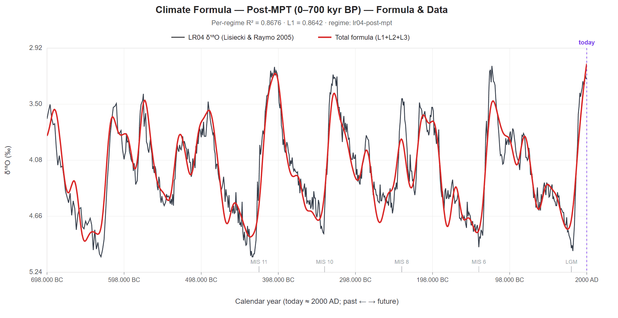
Canonical 3-layer Climate Formula on LR04 δ¹⁸O over the post-MPT window. Red = formula (L1 + L2 + L3, sequential ridge fit); black = observed LR04. R² = 0.780 within this regime — an in-window description, not a prediction (see the T7 note below).
Headline findings
- In-window R² 0.780 post-MPT LR04 — a description of the record; the model’s own orbital histories predict 0.357 of it out of sample (T7). Full per-regime table in §Sequential ridge regression.
- Every significant LR04 peak has a counterpart among the engine’s own beats. 28 beat lines carry the signal; the eigenmode combinations are the same ones Berger names, read from the model’s own integration.
- The 100-kyr glacial cycle is a planetary eigenmode-beat band, not direct Earth-eccentricity forcing. LR04’s 100-kyr band is one broad peak carried by the planets’ eccentricity beats (94.9 / 98.8 / 110.0 kyr), not the split (95k + 125k) structure direct forcing would give. Detail in §The 100-kyr Glacial Cycle.
- Pre-MPT and post-MPT differ in climate sensitivity, not orbital forcing. Per-regime R²: pre-iNHG 0.455, iNHG-MPT 0.609, post-MPT 0.780.
- Frequency-resolved ice-albedo decomposition. Ice-albedo share of total forcing: 54 % at the 100-kyr band, 65 % at obliquity, 65 % at precession, 46 % at long periods (>130 kyr). Both bands the instrument resolves in the older window carry a larger ice share before the MPT than after it (86 % and 98 % at the 100-kyr and precession bands); the obliquity band, where Willeit et al. 2019 makes its sharpest prediction, is not resolvable line by line in a 1-Myr window. Detail in §Ice-Albedo Decomposition and §MPT ice-share shift.
- The forward projection is an extrapolation of the description, not a forecast (T7). The fitted lines extrapolated forward place the next glaciation peak near ~60,500 AD, but lines fitted on one half of a regime window carry no skill on the other half, so that date is what the extrapolation says, not what the model predicts. Detail in §Forward Projection.
Description and prediction are two different numbers (T7, pre-registered). The per-regime R² above are descriptions: the 28 lines sit on the model’s own frequencies, but their amplitudes and phases are fitted inside each regime window, and fitted on one half of a window the same lines have no skill on the other half (hold-out R² −4.50 post-MPT at the shipped ridge; the best any ridge reaches is +0.03). The model’s prediction is the same record regressed on its own orbital histories — e(t), ε(t), e·sin ϖ(t) with one coefficient each and a climate lag of 5.5 kyr: in-window R² 0.378 / 0.458 (post-MPT / iNHG–MPT), and it keeps 0.357 / 0.445 out of sample, above a phase-randomised null (0.257 / 0.380). The gap between the two is one band: post-MPT LR04 carries 0.41 of its variance at 85–135 kyr and a linear response to the orbital histories leaves 0.21 of it unexplained — the 100-kyr band is what the fitted lines describe and no linear forcing predicts. La2004’s histories give the same prediction (0.380). Record: the simulator’s doc 92 §2 and the artifact data/t7-fixed-phase-l1.json.
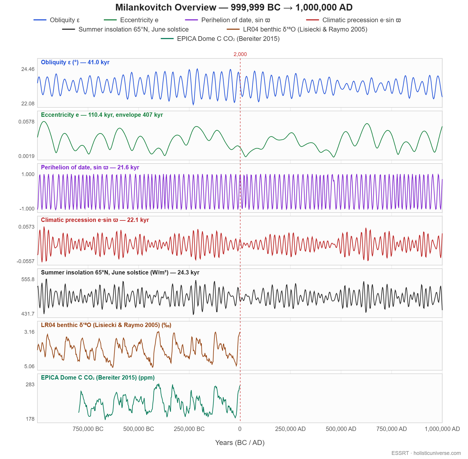
The five upper panels are the model’s own orbital histories, integrated from one cited J2000 state; the two lower panels are the measured records. Everything this page does is the comparison between them — the orbital side is computed without reference to the proxies, and only the per-line amplitudes are fitted.
The canonical three-layer climate formula
Architecture
Computational reference: the shipped line list, per-regime coefficients, denormalization step and validity windows live in the coefficient file public/input/climate-formula-coefficients.json and in doc 92 §2 of the simulator repository; the Python reference implementation is scripts/milankovitch_climate_formula.py. This page is the scientific narrative.
- L1 = 28 lines: 5 climatic-precession beats p+gᵢ, 10 obliquity beats p+sᵢ, 10 eccentricity beats gᵢ−gⱼ, and the 405.6-kyr g₂−g₅ metronome with its 202.8 / 135.2-kyr harmonics — every period Tᵢ from the model’s own N-body modes and precession clock.
- L2 = the carbon-thermostat family — 405 kyr (silicate-weathering thermostat fundamental), 202 kyr (2nd harmonic), 135 kyr (3rd harmonic) — confirmed carbon-amplified across LR04, CENOGRID, EPICA. In the shipped coefficient file this family rides inside L1 and the separate L2 layer is empty.
- L3 = up to 6 Heaviside transitions: PETM (56 Ma), EOT (34 Ma), Mi-1 (23 Ma), MMCT (14 Ma), iNHG (2.7 Ma), MPT (1.0 Ma), applied only when inside the fit window.
- t = age in kyr BP (positive = past, negative = future, t = 0 ≈ 2000 AD); C(t) = normalised δ¹⁸O / δ¹³C / CO₂.
Sequential ridge regression, fit per regime
Coefficients fit by sequential ridge regression: L1 first (ridge λ = 1), then L2 on the residual, then L3 on the L1+L2 residual. Sequential fitting resolves the L1↔L2 collinearity at short windows; ridge resolves the L1↔L1 collinearity among neighbouring lines. The formula is fit independently per climate regime — line periods are the same across regimes; per-line amplitudes and phases vary.
| Regime | Record + window | R² L1 | ΔR² L2 | ΔR² L3 | Total R² |
|---|---|---|---|---|---|
| post-mpt | LR04 0–1 Ma | 0.780 | +0.000 | +0.000 | 0.780 |
| inhg-mpt | LR04 1.0–2.7 Ma | 0.609 | +0.000 | +0.000 | 0.609 |
| pre-inhg | LR04 2.7–5.3 Ma | 0.455 | +0.000 | +0.000 | 0.455 |
| lr04-full | LR04 0–5.3 Ma | 0.325 | +0.000 | +0.008 | 0.333 |
| epica-co2 | EPICA 0–800 kyr | 0.724 | +0.000 | +0.000 | 0.724 |
| cenco2pip | CenCO2PIP 0–66 Ma | 0.047 | +0.000 | +0.644 | 0.692 |
| cenogrid (δ¹⁸O) | CENOGRID 0–67 Ma | 0.004 | +0.000 | +0.613 | 0.617 |
| cenogrid (δ¹³C) | CENOGRID 0–67 Ma | 0.006 | +0.000 | +0.342 | 0.349 |
At Quaternary scales (post-MPT LR04, EPICA CO₂) L1 carries the heavy lifting (R² 0.780 and 0.724 from the orbital lines alone). At deep-time scales (CENOGRID, CenCO2PIP) L3 step transitions dominate (~60% of variance over 67 Myr) — line oscillations average toward zero across many cycles, but discrete step-changes at major transitions carry the deep-time signal.
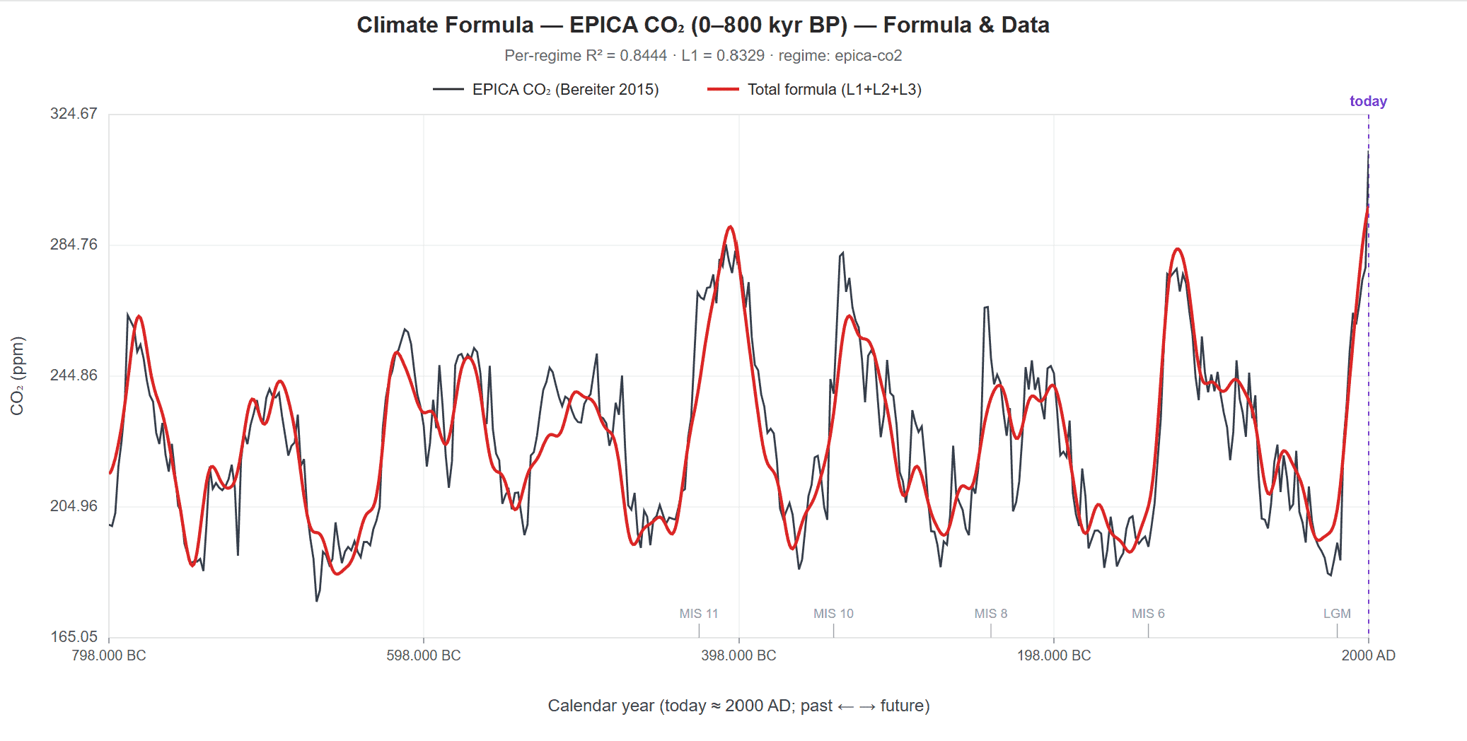
The same line set fitted to atmospheric CO₂ (EPICA Dome C, Bereiter 2015) — independent proxy, independent chronology, entirely different recording physics from benthic δ¹⁸O. R² = 0.724 from L1 alone, 0.724 in total: the orbital structure that describes ice volume also describes atmospheric carbon-cycle dynamics.
Candidates not admitted
- 9-Myr long-period carbon resonance — ΔR² CENOGRID δ¹³C = +0.078 with carbon-amplification ratio 4.2; investigated candidate, cross-window stability test pending.
- Piecewise / polynomial / LOESS detrending — superseded by L3 step covariates (5–10× better R² on CENOGRID).
- Linear-response ODE models for L2 — failed (all L2 ↔ L1 amplitude correlations |r| < 0.4); L2 dynamics are nonlinear (threshold / hysteresis / saturating).
Full inventory: doc 92 §9 .
Try it interactively. The 3D simulation ships with an Earth Climate Analysis modal (Tools menu) that plots the formula reconstruction directly on top of four proxy records across eight tabs: CenCO2PIP · 66M, CENOGRID · 67M, LR04 · 5.3M, LR04 · 1.2M, EPICA · 800k, LR04 · 700k, LR04 · 200k, and LR04 forward (–250 → +250 kyr). Four layer toggles (Proxy data, Total, L1 alone, L2 alone), a per-regime R² breakdown panel, and one Export that prints the view on screen.
The 405-kyr cycle: the engine’s metronome and the carbon thermostat
The ~405-kyr long-eccentricity cycle is the g₂−g₅ beat of the planets’ apsidal modes, and the model’s own N-body engine produces it as the strongest line of Earth’s deep eccentricity spectrum, at 405.6 kyr against the rock record’s 405.6 kyr (Supporting Evidence §14). In the climate record it has a distinct signature.
Carbon-cycle signature. CENOGRID full Cenozoic places the line at 404.5 kyr with FWHM = Rayleigh resolution (clean single-frequency line). The δ¹³C/δ¹⁸O amplitude ratio is 1.53× — vs 0.49 at obliquity and 0.66 at precession. The signal lives preferentially in the carbon record. Phase residuals from a linear orbital model correlate at only r = 0.21 between δ¹³C and δ¹⁸O; about 96% of phase variance evolves independently between the two proxies.
The 405-kyr cycle behaves as an entrained internal oscillator: the silicate-weathering thermostat has a narrow resonance peak near 400 kyr (Walker, Hays & Kasting 1981; Pälike et al. 2006 “heartbeat of the Oligocene climate system”); the long-period orbital eccentricity supplies the energy that synchronises it but does not rigidly drive it. The formula carries it with its 2nd and 3rd harmonics (405 / 202 / 135 kyr). The 9-Myr long-period candidate is investigated but not yet deployed; sub-harmonic (“17 × precession”) alternatives are ruled out by three independent tests, and the g₄−g₃ 2.4-Myr beat shows no comparable carbon-amplification (ratio 0.20 vs 1.53): the thermostat has a narrow resonance peak near 400 kyr, not a broad long-period amplification. In the most recent ~1 Myr of the climate record the 405-kyr component is weak (amplitude ratio 0.12 against the 100-kyr peak — the known “400-kyr problem”), while in the deep record the line is strong and phase-coherent.
The 100-kyr Glacial Cycle
The 100-kyr glacial cycle is a planetary eigenmode-beat band, not direct Earth-eccentricity forcing. LR04’s 100-kyr band is a broad single peak spanning ~80–125 kyr, energy-weighted centroid ≈ 107 kyr — not the split structure (95k + 125k) that direct eccentricity forcing would produce. In the formula the band is carried by the planets’ eccentricity beats read from the model’s own N-body modes — g₄−g₅ at 94.9 kyr, g₃−g₅ at 98.8 kyr, g₃−g₁ at 110.0 kyr among the ten eccentricity lines — whose periods are set by the planets’ masses and distances and do not follow Earth’s spin. The identification is consistent in spirit with Muller & MacDonald 1997 ’s finding that the band lacks eccentricity’s split-peak shape.
Earth’s apsidal period does not drive climate directly
Earth’s own apsidal precession (~111,635 years) is a real cycle but is not a line of the formula and does not play a direct climate-driving role in the 100-kyr world. At T = 1.2 Myr the Rayleigh resolution at P = 110 kyr is ΔP ≈ 10 kyr, so the apsidal period sits within the same broad ~80–125 kyr band as the planetary beats — but the amplitude fit separates them and Earth’s own line drops out. One qualification: in the pre-iNHG regime (2.7–5.3 Myr) the record does carry a line at Earth’s apsidal period — added to the formula there it gives ΔR² = +0.0196, cross-validated, at the model’s own phase (Δφ = −8.5°) — the only position attributable to Earth’s eccentricity rather than to a planetary beat. Its admission to L1 is an open structural decision; see the insolation null test.
Eccentricity attribution has specific empirical headwinds
Direct Earth-eccentricity attribution faces three discriminating empirical failure modes that the planetary-beat reading does not:
| Test | Direct eccentricity attribution | Planetary-beat reading |
|---|---|---|
| 405-kyr term presence (Berger’s strongest predicted eccentricity beat) | Predicts dominant; observed essentially absent in post-MPT LR04 (amplitude ratio 0.12) | The metronome is carbon-amplified and entrained, weak in the recent ice-volume record (above) |
| Eccentricity-beat phase coupling (95k+125k bispectrum) | Predicts strong; not detected (bicoherence 0.507 < null-95 0.555 — replicates Muller & MacDonald 1997) | No contradiction |
| 100-kyr band shape | Predicts the split 95k / 125k pair | One broad peak, centroid ≈ 107 kyr, inside the band of the planets’ eccentricity beats (94.9–110.0 kyr) |
| Berger climatic-precession multi-peak spectrum | Not predicted (these are k+g_j sub-peaks, not eccentricity-beat periods) | Carried directly as the formula’s five p+gᵢ lines |
Ice-Albedo Decomposition
The climate formula’s frequency decomposition makes a quantitative prediction: how much of the temperature signal at each orbital band comes from ice-albedo feedback versus CO₂/greenhouse-gas forcing. Standard paleoclimate references give a single ice-albedo number averaged across the Last Glacial Maximum (Hansen et al. 2013 reports ~3.5 W/m² ≈ 55 % of LGM ΔF). The line fit produces a frequency-resolved decomposition — ice-share separated by orbital band — which has not been published in this form.
Method: Monte Carlo over the four calibration constants — ice fraction f_ice of LR04 δ¹⁸O (default 0.6, range [0.5, 0.7]), sea-level-per-mille ρ_SL (default 120 m/‰, [100, 140]), ice-albedo forcing per metre of sea level κ_F (default 0.04 W/m²/m, [0.030, 0.050]), and the other-GHG multiplier (CH₄ + N₂O + H₂O combined forcing relative to CO₂; default 0.5, [0.4, 0.6]). Per-band amplitude weights come from the L1 fit. Results (post-MPT regime, 0–800 kyr BP):
| Band | Period | Ice-albedo share | Physical interpretation |
|---|---|---|---|
| 100-kyr | 75–130 kyr | 54 % | Ice-sheet feedback dominates post-MPT — consistent with the 100-kyr glacial cycle being an ice-volume signal |
| Obliquity | 35–50 kyr | 65 % | Substantial ice response at obliquity-paced insolation — as predicted by Willeit et al. 2019 |
| Precession | 18–26 kyr | 65 % | High ice-share despite precession being “fast” — reflects ice-sheet response integrated over precession-modulated NH summer insolation |
| Long | >130 kyr | 46 % | CO₂/GHG forcing becomes proportionally more important at long periods (silicate-weathering thermostat regime) |
The decomposition feeds the Charney equilibrium climate sensitivity calculation. Marginalized over the four calibration constants (N = 5,000 MC draws), the ΔT-weighted Charney sensitivity from the frequency-resolved decomposition is 3.35 K, 90 % CI [2.76, 4.01] K — consistent with all major paleo and Bayesian-synthesis estimates (Hansen 2013 , Sherwood et al. 2020 , PALAEOSENS / Köhler et al. 2017 , IPCC AR6). Literature comparison on related work.
The same decomposition computed on the older iNHG-MPT window is the topic of §MPT ice-share shift below.
One mechanism, two observables — the LOD side
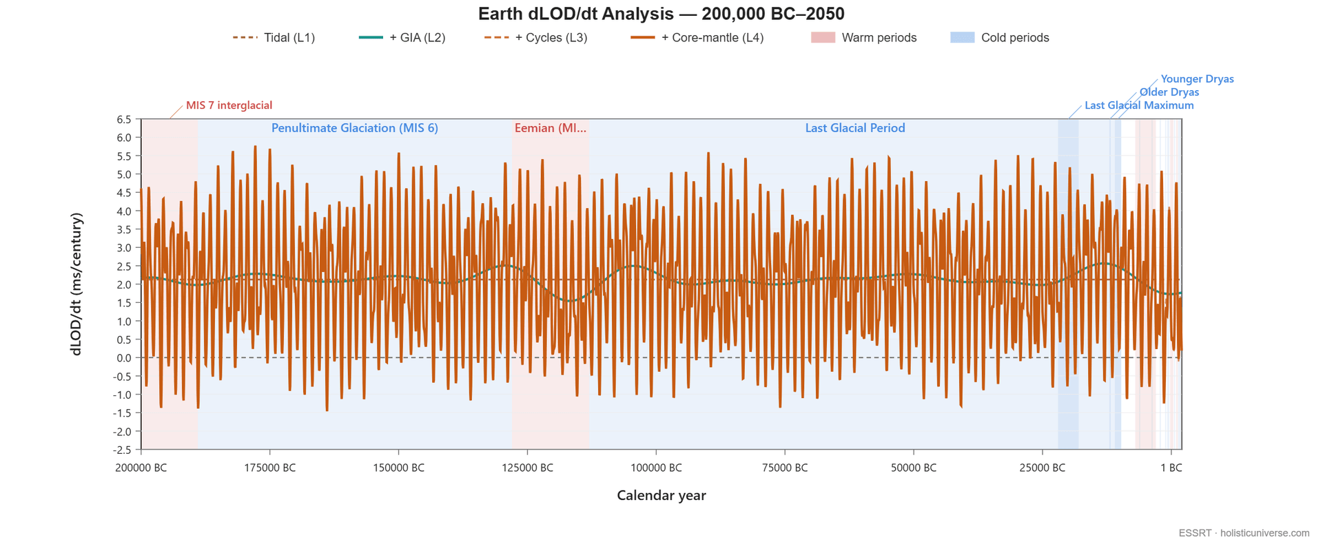
The L1 orbital layer fitted here against LR04 is reused, unchanged, outside climate: it drives the α(t) GIA channel of Earth’s rotation (Timekeeping, Lunar Eclipse Validation §4). Ice sheets grow and retreat under the same orbital forcing; that ice-mass redistribution modulates Earth’s polar moment α; and α modulates the LOD growth rate. The chart below puts both observables on one time axis over the last two glacial cycles. The Tidal + GIA baseline (teal) breathes with the glacial cycle the L1 layer encodes, riding above the tidal line through ice-sheet growth and dipping sharply at the two deglaciations. LR04 itself tracks alongside it — green, inverted δ¹⁸O, the exact dataset this page’s fit targets. The deepest spin-up excursions land at Termination II (→ Eemian) and Termination I (→ Holocene). No LOD data entered the climate fit, and no climate data entered the LOD fit — the alignment is the mechanism.
Pre-MPT vs Post-MPT — same forcing, different response
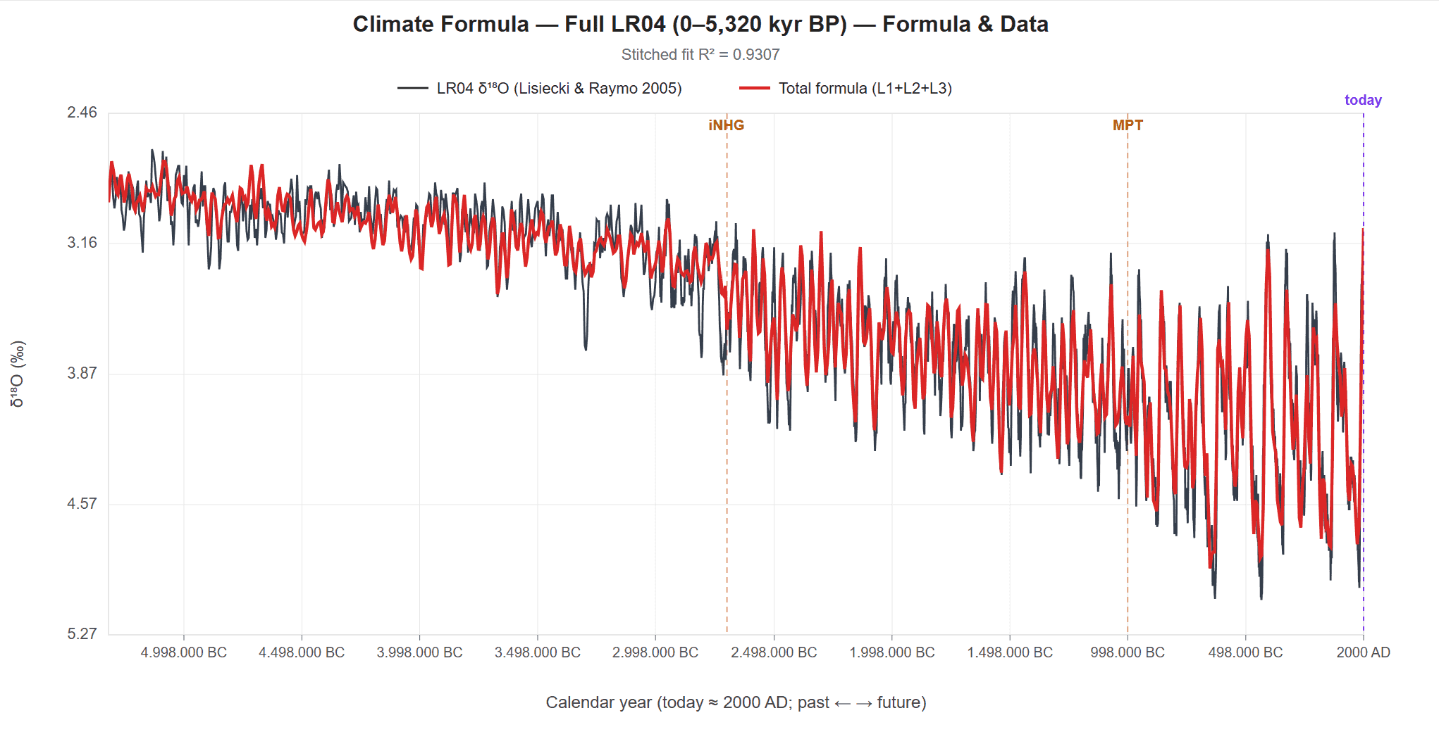
Canonical formula on full LR04 with three independent per-regime fits stitched together. Stitched R² = 0.92. The amplitude growth from left to right is the MPT story: orbital forcing is essentially stationary across 5.3 Myr, but ice-sheet hysteresis amplification grew dramatically after iNHG (~2.7 Ma) and again after MPT (~1 Ma).
Three structural transitions in the full LR04 record: iNHG (~2.7 Ma, Northern Hemisphere ice sheets establish), Early Pleistocene “41-kyr world” (2.7–1.2 Ma, obliquity dominates), MPT (~1.2–0.7 Ma, shift to “100-kyr world” as ice-sheet hysteresis crosses the Willeit threshold).
The orbital forcing — planetary eigenmodes, Earth’s precession, obliquity oscillation — is essentially constant over the past 5 Myr. What changed is the climate system’s sensitivity: long-term CO₂ decline, growing Northern Hemisphere ice sheets, and ice-sheet hysteresis crossing threshold (~1 Ma). The L1 line periods are stationary across the full 5 Myr; per-line amplitudes change across regimes, which is why the formula is fit per regime.
Windowed amplitude analysis across the MPT (pre-MPT 1,500–2,500 kyr vs post-MPT 0–1,000 kyr) gives concrete growth ratios:
| Band | Pre→post ratio | Direction |
|---|---|---|
| 41-kyr obliquity | 0.72× | shrank |
| 100-kyr band | 1.64× | grew |
| 23.7-kyr climatic precession | 2.19× | grew most |
| 405-kyr empirical line (carbon-cycle resonance) | 0.34× | shrank |
The 41-kyr peak decreased — consistent with the standard “ice-sheet saturation silences the obliquity pacemaker” framing (Willeit 2019). The 100-kyr and 23-kyr bands both grew.
MPT ice-share shift
The frequency-resolved ice-albedo decomposition (§Ice-Albedo Decomposition), computed separately on the iNHG-MPT (1–2 Myr BP) and post-MPT (0–800 kyr BP) windows, reads on the shipped line set:
| Band | iNHG-MPT ice share | Post-MPT ice share |
|---|---|---|
| Obliquity (35–50 kyr) | not resolvable line by line | 65 % |
| 100-kyr (75–130 kyr) | 86 % | 54 % |
| Precession (18–26 kyr) | 98 % | 65 % |
Both bands the instrument resolves in the older window carry a larger ice share before the MPT than after it. The obliquity band — where Willeit et al. 2019 ’s “obliquity-paced ice world” makes its sharpest prediction — cannot be read line by line in a 1-Myr window: the formula’s four obliquity lines lie within 2 kyr of each other, below that window’s frequency resolution, and no single line holds a phase against the CO₂ record there. The per-band test of the Willeit picture needs a band-level instrument (the band’s reconstructed signal against CO₂, rather than line by line); it is open.
The older window’s CO₂ comes from CenCO2PIP, a 100-kyr-smoothed reconstruction that biases its ECS high: the iNHG-MPT 100-kyr band reads 7.83 K on CenCO2PIP against 1.63 K on boron-isotope CO₂ (Dyez et al. 2018 ). Post-MPT, where ice-core CO₂ is available, the boron-isotope reconstruction of Chalk et al. 2017 and EPICA agree on the obliquity-band ECS (3.29 K against 2.83 K) and differ at the 100-kyr and precession bands (4.93 against 3.54 K, 4.74 against 3.66 K) — the CO₂ amplitude at those periods is proxy-dependent. Martínez-Botí et al. 2015 and de la Vega et al. 2020 serve the pre-iNHG cross-checks.
Forward Projection
Extrapolating the post-MPT fit forward was withdrawn as a prediction under the pre-registered T7 test: the 28 fitted lines, trained on one half of the window, have no skill on the other half (hold-out R² −4.50; best ridge +0.03), so the extrapolated curve is the description carried forward, not a forecast (Predictions keeps the withdrawn item as the record). The model’s own orbital histories (e, ε, e·sin ϖ) carry the transferable part of the record (0.357 out of sample); a forward projection on them is the honest replacement and has not been computed yet. The line frequencies are the engine’s own beats and transfer; it is the fitted amplitudes and phases that do not.
Limitations
Within-regime descriptive power is high; predictive power is zero both across regimes and within them — formulas trained on pre-MPT data give catastrophically negative R² when applied to post-MPT, and vice versa, and (T7) lines trained on one half of a regime window give negative R² on the other half. The forward projection inherits this. The L1 line periods are regime-independent, but per-line response amplitudes evolve with boundary conditions (CO₂, ice-sheet area). Forward projection therefore stays in scope only within the post-MPT regime (no scheduled boundary-condition shift in the next 250 kyr).
Anthropogenic CO₂ may delay the next natural glaciation by 50+ kyr in moderate-emission scenarios (Ganopolski et al. 2016 ) or up to ~100 kyr in high-emission scenarios. Not modelled here.
The Insolation Null Test
Does adding the classical Berger 1978 insolation features — obliquity ε(t), eccentricity e(t), and the climatic-precession products e·sin(ϖ), e·cos(ϖ) — to L1+L2+L3 improve R²? If yes, they earn a fourth canonical layer; if no, the lines already encode whatever insolation contributes. The features were extracted at LR04 sample times, standardised, and fitted to the L1+L2+L3 residual by ridge regression, with a pre-registered rule: max ΔR² > 0.02 adopt · 0.005–0.02 investigate stability · < 0.005 null. The features are the model’s own Earth orbit — the N-body eccentricity series, the obliquity hybrid and the longitude of perihelion of date — and the baseline is the shipped 28-line formula.
| Regime | Window (kyr) | L1+L2+L3 | + L_insol | ΔR² |
|---|---|---|---|---|
| post-MPT | 0–1000 | 0.7805 | 0.7821 | +0.0017 |
| iNHG-MPT | 1000–2700 | 0.6090 | 0.6095 | +0.0005 |
| pre-iNHG | 2700–5320 | 0.4547 | 0.4611 | +0.0064 |
| lr04-full | 0–5320 | 0.3329 | 0.3522 | +0.0193 |
| EPICA CO₂ | 0–800 | 0.7238 | 0.7244 | +0.0006 |
On their own, the classical features explain very little of the ice-volume record:
| Regime | R²_L1 | R²_insol_only | L1 / insol ratio |
|---|---|---|---|
| post-MPT | 0.780 | 0.2362 | 3× |
| iNHG-MPT | 0.609 | 0.1665 | 4× |
| pre-iNHG | 0.455 | 0.0939 | 5× |
| lr04-full | 0.325 | 0.1167 | 3× |
Substituting an independent orbital solution (La2010a on 0–500 kyr; La2004 over the full record) gives the same reading as the model’s own orbit:
| Test | LR04 (0–500 kyr) | EPICA CO₂ (0–500 kyr) |
|---|---|---|
| L1+L2+L3 (canonical formula) | R² = 0.8690 | R² = 0.8236 |
| Berger insolation alone (Laskar e/ϖ) | R² = 0.202 | R² = 0.129 |
| L1+L2+L3 + Berger insolation (Laskar) | ΔR² = +0.00758 | ΔR² = +0.00794 |
Verdict: no fourth layer. The pre-registered rule adopts the layer only on a cross-window-stable gain above 0.02, and no window reaches it. Every regime window is negative out of sample; the full 5.3-Myr record is the one window with an out-of-sample gain — −0.0356 with the model’s features, −0.0389 with La2004’s — inside the tentative band, below the bar (its in-sample +0.0193 does not hold out of sample). The 0–500 kyr readings above are in-sample values on a window whose enclosing regime cross-validates negative. The model’s own orbit and La2004 read alike in every regime, as expected for two integrations of the same secular system.
The strict mathematical reading: the L1 frequencies (the p+gᵢ, p+sᵢ and gᵢ−gⱼ beats) span, at the linear level, the same subspace as Berger’s 4-feature decomposition — once L1 is in the model, the Berger features add only what 28 fixed-frequency lines leave un-spanned on a given window, and the cross-window check shows that remainder is not stable. Only the four linear Milankovitch features were tested; higher-order Berger terms are products and harmonics of the same primitives. Reproducibility: three deterministic scripts and three tracked result files in the 3d repository ; every number above is bound to them.
The Present Era in the Formula
The 405-kyr carbon-thermostat line sits near a warming peak around the present era — a fitted observation from LR04 (the line’s phase is set by the regression; the cycle position falls where it falls): amplitude ~0.5–1.0 °C peak-to-trough post-MPT, rate of change at peak < 0.005 °C/century. Two natural-cycle signals therefore point opposite directions for the current era: the precession-driven NH summer insolation (~23.7 kyr) has been declining since the Holocene Climate Optimum (~10 kyr BP) — the standard “natural cooling trend” — while the 405-kyr thermostat puts the natural baseline slightly warmer than the long-term mean. Both are real, at different timescales; mainstream Holocene attribution emphasises the first, and the second is rarely cited outside cyclostratigraphy — one quantitative element for the active “Holocene Temperature Conundrum ” debate.
Bounded conclusions only. The thermostat line’s rate of change (< 0.005 °C/century at peak) is ~300× too slow to explain industrial-era warming (~0.7 °C/century): the current-era peak affects the baseline level, not the recent rate. The framework is descriptive within regimes, not predictive across boundary-condition shifts.
Related Work
The framework sits within the active wave of revisions to classical Milankovitch theory, and adds two contributions not found in the surveyed literature: the lines as the engine’s own secular beats with frequencies fixed before any fit, and the insolation null test (above).
- Dutkiewicz et al. 2024 (Nat. Commun.) — the closest precedent: identifies Mars–Earth gravitational resonance (g₄−g₃, 2.4 Myr) as a direct climate driver in 65 Myr of deep-sea hiatus data, framed as gravitational forcing rather than insolation. Same mechanism and direction of causation as the framework — which carries 28 beats of one N-body mode table where Dutkiewicz documents one.
- Zeebe & Lantink 2024 (AJ) — states that the ~405-kyr-metronome paradigm “requires revision” (the σ₁₂ resonance can disrupt g₂−g₅). The model’s own engine produces the metronome from gravity alone and treats its climate expression as an entrained carbon-cycle response rather than a rigid drive; both readings may hold simultaneously.
- Wunsch 2003 / Roe 2006 — the orbital-vs-stochastic debate. The formula’s in-window R² = 0.780 on post-MPT LR04 is incompatible with Wunsch’s red-noise null and consistent with Roe’s defence, from a different parameterisation basis that makes the channel question explicit; T7 bounds how much of that is description.
- Boulila 2019 (Sci. Rep.) — the ~9-Myr Grand cycle; the framework does not promote a 9-Myr line (a stability test finds no single coherent oscillator), consistent with a multi-mechanism reading.
- Cyclostratigraphy (Hinnov 2018 ; Acycle; Imbrie & Imbrie → Huybers) — the methodological neighbour: multi-tone sinusoidal regression routinely reaching R² 0.6–0.9 on post-MPT records. The framework’s difference is structural: the beat frequencies are read from the model’s own N-body modes and precession clock rather than fitted per record, and 405 kyr is treated as a carbon-cycle response rather than the universal anchor.
- Munk et al. 2002 — named the disciplinary gap between the tidal community (periods ≤ 18.6 yr) and the Milankovitch community (≥ 20 kyr); the gravitational-coupling framing closes it: one source, two channels.
Climate sensitivity. The frequency-resolved ice-albedo/CO₂ decomposition (above) yields Charney ECS = 3.35 K, 90 % CI [2.76, 4.01] K — inside all four published reference ranges, from an orthogonal, frequency-domain direction:
| Source | Charney ECS (K) | Method |
|---|---|---|
| This framework (frequency-domain line decomposition, MC) | 3.35 [2.76–4.01] | frequency-domain decomposition |
| IPCC AR6 | best 3.0 (likely 2.5–4.0) | multi-line synthesis |
| Sherwood et al. 2020 | 2.6–3.9 (66 % CI) | Bayesian synthesis |
| Hansen et al. 2013 | 3.0 ± 0.5 | LGM-to-Holocene time-domain |
| PALAEOSENS / Köhler et al. 2017 | 3.0–4.5 | multi-proxy paleo |
The per-band ice-share decomposition (54 % at 100 kyr, 65 % at obliquity, 65 % at precession) and its per-window reading across the MPT (§MPT ice-share shift) are a product none of the reference methods produce.
Methodology highlights
| Topic | Detail |
|---|---|
| Spectral methods | MTM (Thomson multitaper, NW=3, K=5); Lomb-Scargle for Cheng2016’s irregular sampling; Hinich bispectrum for eccentricity-beat coupling; multi-component OLS for amplitude fit; single-component OLS for the line scan |
| Rayleigh resolution | ΔP ≈ P²/T. At T = 5,320 kyr (full LR04) and P = 41 kyr: ΔP ≈ 0.32 kyr (Berger sub-peaks resolvable). At T = 1.2 Myr and P = 110 kyr: ΔP ≈ 10 kyr (95k/100k/112k spectrally collinear). |
| Pre-registration | Every empirical test had data source, method, parameters, and verdict rules locked in writing before any data analysis |
| Bootstrap | 1,000 resampling iterations for amplitude confidence intervals |
Reproducibility scripts: 3d repository .
Data sources
- LR04 stack — Lisiecki & Raymo 2005 , Paleoceanography 20, PA1003. 57 benthic δ¹⁸O records, 0–5,320 kyr BP. Primary spectral analysis; per-regime L1+L2+L3 fits.
- CENOGRID composite — Westerhold et al. 2020 , Science 369, 1383. Cenozoic δ¹⁸O + δ¹³C global composite, 0–67 Myr BP. Deep-time L3 step generalization.
- EPICA Dome C CO₂ — Bereiter et al. 2015 , Geophys. Res. Lett. 42, 542. Antarctic ice-core atmospheric CO₂, 0–805 kyr BP. Cross-proxy validation.
- CenCO2PIP CO₂ — Consortium 2023 , Science 382, eadi5177. Bayesian multi-proxy CO₂ synthesis, 0–66 Ma. Deep-time CO₂ validation.
- Cheng 2016 Asian speleothem composite — Cheng et al. 2016 , Nature 534, 640. U-Th-dated Asian Monsoon δ¹⁸O, 0–640 kyr BP. Non-tuned chronology-bias control.
See also
N-body Exploration · Obliquity & Inclination · Eccentricity · Why Earth Is Special · Supporting Evidence §1 (100-kyr problem + ice-core dating methodology) · Earth’s Clock