Predictions
The Holistic model produces specific testable predictions that differ from conventional theory and can be checked against future observations. Predictions are grouped by timeline.
All predictions are measured from the 3D model. Every value on this page is read directly from the 3D Simulation using objective measurement functions — not derived from theoretical assumptions. See Analysis & Export Tools for how measurements are taken.
Near-term predictions (decades)
1. Mercury’s “missing” perihelion precession will decrease
Mercury’s perihelion precession includes a ~43″/cy contribution attributed to General Relativity. The model attributes this to Earth’s wobble on its Axial Precession Orbit rather than space-time curvature. The geocentric rate should therefore decrease — by ~5.0″/century:
| Year | Geocentric (moving equinox) | Heliocentric (ICRF) | “Anomaly” |
|---|---|---|---|
| 2000 AD | ~5,598.25″ | ~569.45″ | ~38.01″ |
| 2100 AD | ~5,592.84″ | ~564.04″ | ~32.60″ |
Falsifiability: if geocentric precession stays constant at ~5,604″/cy → standard GR supported; if it decreases from ~5,598.25 toward ~5,592.84″/cy → the model is supported.
Near-term test — BepiColombo: Mercury orbit insertion 21 November 2026; routine science from April 2027. The MORE instrument will measure Mercury’s orbit at 1–2 orders of magnitude better precision than MESSENGER. The model predicts ~574.61″/cy or lower vs MESSENGER’s 575.31″/cy — a 0.70″/cy difference, ~500× larger than MESSENGER’s uncertainty. The test is decisive if BepiColombo’s pipeline reports the raw measured perihelion advance rather than a GR-inclusive ephemeris fit total — methodology canonical at Mercury Precession §BepiColombo Test.
2. RA at maximum declination will shift from 6h
Coordinate-system note: in standard precessing equatorial coordinates the June solstice is at RA 6h by definition. This prediction refers to the Sun’s position in a fixed reference frame (ICRF) at maximum declination.
The Sun’s ICRF position at June solstice peaked at exactly 6h in 1246.03125 AD and is now slowly shifting. By ~6,000 AD it will be ~5h58m22s.
| Property | Value |
|---|---|
| Mean RA at max declination (fixed frame) | ~5h48m50s / ~17h48m50s |
| Oscillation amplitude | ±11 minutes |
| Cycle period | ~41,915 years |
| Peak value | ~6h00m00s (reached in 1246.03125 AD) |
| Predicted value by 6,000 AD | ~5h58m22s |


Current shift rate ~17 arcsec/century, well within modern astrometric precision. The mechanism and amplitude are independently confirmed by standard IAU 2006 precession theory: m_A = p_A × cos(ε) − χ_A inherits the obliquity period because it depends on cos(ε) (Capitaine et al. 2003 ; Laskar et al. 1993 ). A back-of-envelope calculation gives ~±10 minutes of RA — matching the model’s ±11 minutes. Canonical: Supporting Evidence §7.
3. Jupiter and Saturn perihelion trends will continue
WebGeocalc displays apparent pattern changes for Jupiter and Saturn perihelion precession over the next centuries. The model predicts the current trends continue as-is — Jupiter prograde at perihelion period 8H/39 = 68,783 yr and Saturn retrograde at −8H/65 = 41,270 yr (8H-lattice secular periods). Saturn’s observed ecliptic-retrograde rate ~-3,400″/cy (WebGeoCalc) is consistent with the model.


The disagreement: standard theory attributes Saturn’s ecliptic-retrograde motion to a transient phase of the Great Inequality (~883-yr oscillation from the 5:2 resonance), reversing within ~450 years. The model treats it as permanent. For Jupiter the disagreement is in period — secular theory implies ~305,000 yr vs the model’s 68,783 yr; Jupiter’s observed inclination trend favours the shorter period (~3″/cy error vs ~8.5″/cy). Full analysis: Supporting Evidence §12 and §8.
4. No major Planet Nine (key differentiator)
The Batygin–Brown hypothesis posits an undiscovered 4–10 M_Earth planet at 290–700 AU shepherding extreme TNOs. A two-tier test against the model rejects all proposed candidates: (primary) Law-4 compliance — the observed eccentricity must match e_amp = K · sin(tilt) · √d / (√m · a^(3/2)); all proposed candidates fail by 4–7 orders of magnitude. (secondary) v-balance — adding a 9th body crashes the canonical closure for any mass above ~10⁻⁴ M_Earth. Combined threshold for compatibility at high-e ETNO orbits: ~2 × 10⁻¹⁰ M_Earth (~2-km rocky asteroid).
| Candidate | Mass (M_E) | Distance (AU) | Best 9-planet balance | Verdict |
|---|---|---|---|---|
| Batygin & Brown 2016 | 10.0 | 700 | 1.25% | REJECT |
| Brown & Batygin 2021 | 6.2 | 380 | 10.07% | REJECT |
| Siraj et al. 2025 | 4.4 | 290 | 13.19% | REJECT |
| Pluto-mass test | 0.0022 | 460 | 94.71% | MARGINAL |
| Ceres-mass test | 0.00016 | 460 | 99.99% | ACCEPT (v-balance only) |
Under the primary Law-4 test, even the Ceres-mass candidate fails (its eccentricity 0.25 is 4,270× larger than the maximum Law-4 amplitude). Verdict: no candidate at proposed parameters is framework-compatible.
Near-term test — Vera Rubin Observatory (LSST 2025–2035):
| LSST outcome | Model prediction | Conventional Batygin/Brown |
|---|---|---|
| M ≥ 1 M_Earth at 300–700 AU, e ≈ 0.2–0.6 | FALSIFIED | confirmed |
| Ceres-mass body at 300–500 AU, high e | FALSIFIED | weakened |
| Tiny body (≲ 2 × 10⁻¹⁰ M_Earth) at similar orbit | consistent | n/a |
| No detection above ~10⁻¹⁰ M_Earth by 2035 | consistent | FALSIFIED |
| ETNO clustering disappears with more discoveries | consistent | FALSIFIED |
A single detection of any ≳ Ceres-mass body in a high-e Batygin–Brown-style orbit falsifies the model. The conventional hypothesis can be re-parameterised to fit nearly any detection — making it harder to falsify cleanly. In Popper’s terms, the model’s prediction is more vulnerable and therefore stronger. Full search, ETNO data, and alternative explanations: Planet Nine.
5. Small classical-belt KBO obliquity clustering (Law 4 bidirectional)
Law 4 is bidirectional. Solving the closure for sin(tilt) gives an obliquity prediction from a body’s mass, semi-major axis, eccentricity amplitude, and Fibonacci d-slot:
sin(tilt) = e_amp · √m · a^(3/2) / (K · √d)
For the 8 IAU planets this closes to <1%. For a representative 100-km classical-belt KBO at a ≈ 45 AU, e ≈ 0.05, mass ~10⁻¹² M☉, Law 4 predicts axial obliquity ≈ 36.6° at d = 55. The population-statistical claim: small cold-classical-belt KBOs (the regime where external forcing on e_amp is weakest) should cluster near this prediction, rather than show the uniform-random ~57° mean expected from Lambert’s law on a sphere.
| LSST outcome (~10³ small-TNO rotation-pole measurements by 2030–2035) | Verdict |
|---|---|
| Small classical-belt KBO obliquities cluster near ~30°–50° | Bidirectional Law 4 confirmed beyond the 8 planets |
| Obliquity distribution is uniform-random (~57° mean) | Bidirectional reading restricted to the 8-planet domain |
The ~30% gap between the model prediction (~36.6°) and the random expectation (~57°) is resolvable with ~10² obliquity measurements at ±10° precision.
Scope caveat: no individually named TNO is per-body testable — every catalogued/named TNO (Pluto, Eris, Haumea, Makemake, Quaoar, Sedna, …) is too large at its observed eccentricity to be Law-4-admissible. Comets and main-belt asteroids fail too (Jupiter scattering, outgassing, Yarkovsky/YORP). The framework’s positive predictive zone is the sub-200 km low-e cold-classical-belt population (10⁴–10⁵ bodies enumerated by Col-OSSOS), tested statistically across many rotation-pole measurements.
Law-4 closure ≡ “cleared the neighborhood”: the framework’s planet/non-planet partition coincides with the IAU’s 2006 third criterion. Soter (2006) proposed a mass-discriminant Λ but it never became canonical; Law-4 closure provides a different quantitative formalisation that returns a clean pass/fail and matches the same 8-body partition. Agreement is not tautological: Planet Nine candidates fail Law-4 closure by 4–7 orders of magnitude (prediction #4), and the small-KBO obliquity-clustering signature here is the second non-circular extension.
Medium-term predictions (centuries)
6. Obliquity
Standard theory: obliquity (23.4393° in 2000 AD) decreases until ~13,900 AD, reaching ~22.6° (Chapront et al. & Laskar). The model agrees through ~13,700 AD; the next obliquity minimum lands at ~22.51° around year 13,665 AD, after which obliquity rises again on the ~41,915-year cycle. Both bottom out near the same epoch; they differ on what happens next — the model predicts a clean reversal back toward the mean; polynomial extrapolations diverge.
The full long-term envelope is ~22.21° – ~24.72°, with the high end (~24.72°) sitting slightly above Laskar’s standard maximum (~24.5°) — a distinct prediction worth testing against paleoclimate proxies.

7. Longitude of perihelion
The model matches Meeus’s formula closely until ~3000 AD; afterward the two diverge. The model completes 360° in a mean period of ~20,957 yr; Meeus’s polynomial extrapolation deviates increasingly outside its fit window.


8. Gregorian calendar drift
The Gregorian year (365.2425 days) doesn’t match the actual solar year (~365.2422036 days):
- By 6486 AD: June solstice on June 17, 20:00 UTC
- By 11,725 AD: June solstice on June 17, 10:00 UTC (4 days earlier than today)
9. Analemma shape changes
The analemma shifts forward in time with the perihelion precession cycle. Its width changes with eccentricity (~20,957-year cycle); its length changes with obliquity (fluctuating between 22.21° and 24.72°).

10. Axial precession period reaches a minimum, then increases
Current Capitaine polynomial: axial precession period is decreasing. The model agrees on the current trend but predicts a reversal: minimum of ~25,312 yr around year 12,431 AD, then a rise to ~26,051 yr around year 32,341 AD, then continued oscillation on the perihelion precession cycle. The Capitaine polynomial does not model this oscillation. The underlying cause is the interaction between lengthening day and shortening solar year.
On geological timescales, the mean itself drifts. The model’s H/13 axial precession period was ~5,372 yr at Hadean, ~23,776 yr at Devonian, ~~25,794 yr today, and rises to ~26,974 yr at +200 Myr. The classical “precession of the equinoxes” — known since Hipparchus and traditionally treated as a fixed astronomical constant — is a now-snapshot of an H(t)-evolving cycle. The modern rate of change is ~0.5 yr per Myr: small but in principle observable in high-precision IAU precession-rate measurements over decades. Framework: Expanding Resonance.

Long-term predictions (millennia)
11. Eccentricity (key differentiator)
Standard theory: Earth’s orbital eccentricity (0.01671 in 2000 AD) decreases toward ~0 by ~27,000 AD. The model predicts it reaches a minimum of ~0.0140 much earlier — around year 11,725 AD — and then increases again. Canonical: Eccentricity.

12. Inclination
Standard theory: Earth’s inclination to the invariable plane (1.57869° in 2000 AD) decreases, with no minimum predicted. The model predicts inclination decreases to ~0.845° in year 32,682 AD, then increases again on the ~111,772-year cycle.

13. Earth rotation / LOD / Delta-T
Standard theory: Earth’s rotation is monotonically slowing due to tidal friction. The empirical Stephenson polynomial encodes a non-tidal Earth-rotation speedup component (the Munk-MacDonald hypothesis) on top, attributing the gap between pure-tidal prediction and the historical eclipse record to glacial isostatic adjustment + core-mantle coupling. The model predicts LOD will increase until ~30,000 AD, then decrease until ~2,000 AD, before increasing again — short-term fluctuations (like the 2020–present speedup) sit on top of this trend. Both sidereal day and stellar day follow the same cyclical pattern. The model’s pure-tidal ΔT formula has been empirically confirmed against 19 documented historical solar eclipses spanning -762 to 1654 CE (19/19 events visible at the documented site vs Stephenson empirical fit’s 17/19) — no non-tidal-speedup component is required by the historical record. Canonical: Timekeeping; empirical validation: Historical Eclipse Validation.

14. Solar year length in days
Laskar: solar year in days decreases until ~10,900 AD (assuming a fixed 86,400-second day). The model: decrease until 30,000 AD.

15. Sidereal year in seconds
Chapront et al.: slowly increasing until ~15,600 AD. The model: fixed at 31,558,149.76 seconds — the anchor point of the entire framework.
16. All precession movements are related
Standard theory treats ecliptic, axial, and other precession motions as largely unrelated. The model predicts they all follow a clear pattern repeating every ~20,957-year perihelion cycle.

Structural predictions
17. Invariable plane tilt
Earth’s path relative to the invariable plane has mean tilt ~1.48113° with amplitude ~0.63603°. The same structure governs all planetary motion: Jupiter’s precession determines Earth’s ecliptic precession, Saturn’s precession determines Earth’s obliquity cycle.


Saturn is the only planet whose perihelion precesses retrograde in the ecliptic frame (confirmed by JPL WebGeoCalc at ~-3,400 arcsec/cy — canonical at Supporting Evidence §12) and the only anti-phase planet (cosine sign flipped). Saturn alone carries the entire anti-phase side; the seven other planets form the in-phase group. The angular-momentum-weighted inclination amplitudes cancel between groups to 99.9974%, keeping the invariable plane balanced; the same partition independently satisfies the eccentricity balance (99.8636%). Full derivation: Fibonacci Laws Derivation §Law 3. Visualise via Tools > Invariable Plane Inspector in the 3D Simulation .
Climate prediction
18. Next natural glaciation peak at ~60,500 AD
The canonical 3-layer Climate Formula extrapolated forward from t ≈ 2000 AD identifies the next predicted glacial maxima and interglacial peaks:
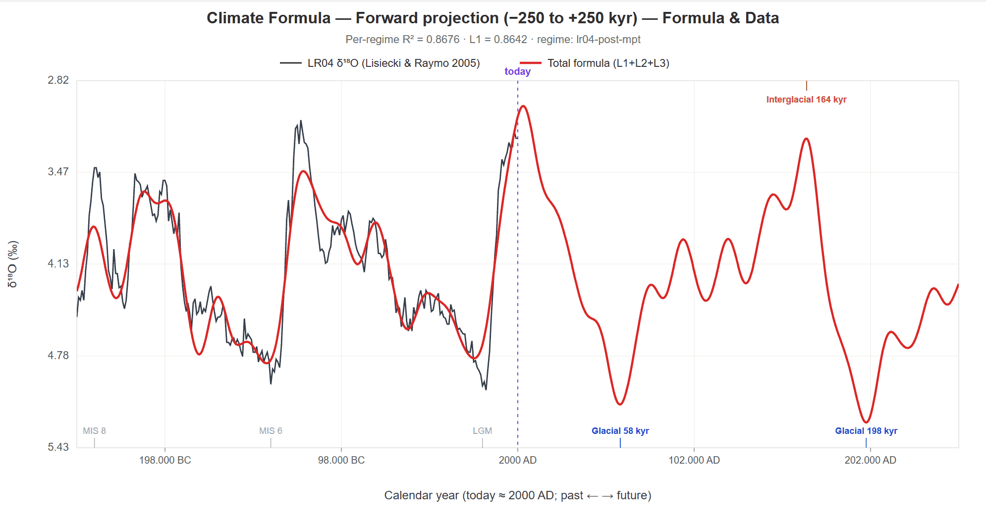
| Years from now | AD date | C(t) normalized | Note |
|---|---|---|---|
| ~58,500 | ~60,500 AD | +2.27 | Next natural glaciation onset |
| ~106,000 | ~108,000 AD | +0.24 | mild |
| ~153,000 | ~155,000 AD | −0.99 | (local max, interglacial-range) |
| ~164,000 | ~166,000 AD | −2.31 | Warmest interglacial in window |
| ~196,500 | ~198,500 AD | +2.48 | Strongest glaciation in next 250 kyr |
The signal C(t) is the normalised δ¹⁸O proxy from the post-MPT regime fit (negative = warmer/interglacial; positive = colder/glacial). The Holocene is correctly identified as interglacial; MIS 6 is placed within ~2 kyr; the LGM is predicted within ~9 kyr (the expected ice-sheet response lag).
Comparison with established forecasts:
| Framework | Next glacial onset (kyr from now) | Mechanism |
|---|---|---|
| Berger & Loutre (2002) | ~50 | Astronomical insolation + LLN-2D climate model |
| Loutre & Berger (2003) | ~50–100 | Same + low-CO₂ scenarios |
| Tzedakis et al. (2012) | ~50 (analog-bound) | MIS 19c past-interglacial analog |
| Ganopolski et al. (2016) | ~50 (no CO₂) / ~100 (moderate) / ≥500 (high) | CLIMBER-2 with explicit CO₂ feedback |
| Holistic Climate Formula | ~58 | 32-integer 8H lattice + L2 carbon thermostat + L3 step transitions |
The Holistic ~58.5 kyr (~60,500 AD) prediction sits in the consensus range and matches Berger & Loutre 2002 within ~16%. What distinguishes it is the mechanism: standard frameworks attribute the 100-kyr cycle to direct eccentricity forcing; the model attributes it to the s₁ − s₄ nodal eigenmode beat at n = 25 = 107.3 kyr — a planet-pair orbital-plane coupling. Full comparison and mechanistic distinction: Climate Formula.
Orbital forcing is not climate: the formula captures the orbital component (L1) + silicate-weathering thermostat (L2) + discrete Cenozoic step transitions (L3). It does not model ice-sheet hysteresis, CO₂ amplification feedbacks beyond L2, regional asymmetries, or anthropogenic CO₂. The ~58,500 yr glacial-onset prediction is when the orbital clock makes a phase transition possible, not when surface climate necessarily follows — ice sheets carry thermal memory. Ganopolski et al. (2016) found moderate-emission anthropogenic CO₂ may delay the next natural glaciation by 50+ kyr (high-emission ≥100+ kyr).
The pacing departs from the post-MPT 100-kyr regime: two strong glaciations at ~58.5 kyr and ~196.5 kyr from now (138 kyr apart, not the regular ~100-kyr drumbeat), with mostly weak intermediate wiggles. The L1 orbital component is exactly 8H-periodic and matches the late-Pliocene “41-kyr world” 8H ago. Physical interpretation and three climate-response scenarios: Climate Formula §Pacing shift.
19. Planet obliquity cycles (two-component structure)
Every planet with an obliquity cycle follows the same two-component formula as Earth — the sum of two cosines with equal amplitude, one at the ICRF perihelion period and one at the obliquity cycle period:
obliquity(t) = mean − A × cos(ICRF period) + A × cos(obliquity cycle)
Three obliquity cycles are already confirmed:
| Planet | Predicted cycle | Observed | Error | Source |
|---|---|---|---|---|
| Mercury | 894,179 yr (8H/3) | ~895,000 yr | 0.2% | Bills & Comstock 2005 |
| Earth | ~41,915 yr (H/8) | ~41,000 yr | 2% | Laskar+ 1993 |
| Mars | 127,740 yr (8H/21) | ~124,800 yr | 2.4% | Ward 1973; Laskar+ 2004 |
Three remain testable:
| Planet | Predicted cycle | Current literature | How to test |
|---|---|---|---|
| Jupiter | 167,659 yr (H/2) | “No regular cycle” (Saillenfest+ 2020) | Long-term spin-axis integration |
| Saturn | 111,772 yr (H/3) | “No regular cycle” (Saillenfest+ 2021) | Long-term spin-axis integration |
| Uranus | 167,659 yr (H/2) | “Frozen at ~98°” (Saillenfest+ 2022) | Extremely long timescale simulation |
Venus and Neptune have obliquity cycle = |ICRF perihelion period| (auto-derived from their ecliptic periods, tidally damped). The two-component formula cancels exactly, producing constant obliquity — consistent with observations (Venus 177°, Neptune ~28°). Two-component formula canonical at Obliquity §A Universal Pattern.
Deep-time predictions
These predictions extend the model’s testable claims across geological time, from Earth’s Hadean origin through the modern epoch to the far-future tidal-lock asymptote. They follow from the proper-physics two-layer LOD formula (Driver 1 — Earth-Moon tidal evolution) combined with the adiabatic invariant a × M_☉ = const (Driver 2 — solar mass loss). Framework: Expanding Resonance.
20. Hadean Moon at the Roche limit
At Patterson’s Pb-Pb radiometric Earth age of 4.54 Gyr, the proper-physics two-layer LOD formula places the Moon at 20,532 km = 3.22 R_E — just outside the Roche limit (~2.9 R_E, where a fluid Moon would tidally disintegrate). No Hadean constraint was used in the fit; the formula is anchored at modern LOD = 24 hr and calibrated against Farhat 2022’s Phanerozoic deep-time tidal-evolution curve. Any future radiometric or paleoclimate technique that refines either Earth’s age or the Hadean Moon distance should remain consistent with this match. A measured Hadean Moon distance outside ~2.5–5 R_E at Patterson’s epoch falsifies the prediction.
21. Devonian H ≈ 309,083 yr matches Wells 1963 to within 1 %
The model’s Devonian (380 Ma) Earth Fundamental Cycle is H = 309,083 yr, producing 396.21 tropical days/year — matching Wells 1963’s directly-counted Devonian coral growth rings (~400 days/yr) to within 1 %. New high-precision paleontological day-count techniques (expanded Torreites bivalve sampling, recalibrated coral growth-band analysis, tidal-rhythmite inter-annual cycles) should reproduce this match. A measured Devonian count outside ~390–405 days/yr falsifies the prediction. Canonical validation table: Supporting Evidence §14.
22. Integer-label invariance across geological time
The L1 lattice integers (n = 65 for the climate-recorded obliquity main beat, n = 39 for Jupiter’s ecliptic perihelion, n = 16 for Earth’s perihelion harmonic, and the full 32-integer set) are structural constants of the solar system’s secular dynamics. The absolute periods rescale as H(t) expands across geological time, but the integer labels themselves do not change. Independent cyclostratigraphic L1 lattice fits to Devonian, Permian, and Cretaceous proxy spectra should find the same set of integers identified in the post-MPT LR04 fit — only with rescaled absolute periods. A deep-time spectrum that fits a substantively different integer set (e.g., a Devonian lattice missing n = 65 or with a new structurally-dominant integer absent post-MPT) falsifies the framework’s invariance claim.
23. Future tidal-lock asymptote at 87.1 R_E
The Earth-Moon system asymptotically approaches tidal lock at Moon distance 555,623 km = 87.1 R_E (currently 60.3 R_E), reached at roughly 50 Gyr from now — well beyond the proper-physics formula’s +3 Gyr predictive horizon and beyond the Sun’s red-giant phase at +5 Gyr. Lunar laser ranging extrapolated forward through full tidal-Q decay should converge on this angular-momentum boundary. A converged asymptote outside ~80–95 R_E falsifies the angular-momentum calculation.
24. Cheng cross-proxy persistence
The L1 lattice currently fits Cheng 2016’s Asian-Monsoon δ¹⁸O record at R² = 0.68 on its independent U-Th radiometric chronology (see Supporting Evidence §13). As new high-precision speleothem chronologies extend the record or refine its dating, the same 32-integer lattice should continue to fit with comparable R². A substantially degraded fit (R² dropping below ~0.5 on a refined or extended Cheng record) would falsify both the lattice’s cross-proxy persistence and the integer-label invariance claim above (§22).
Verification pathways
| Prediction | Timeframe | Type |
|---|---|---|
| Mercury geocentric precession decrease | Decades | Differs from GR |
| RA shift from 6h | Centuries | New observable |
| Jupiter/Saturn perihelion trend | Decades | Differs from WebGeocalc |
| No major Planet Nine (Law-4 compliance, ≳ 2 × 10⁻¹⁰ M_Earth at high-e ETNO orbits) | Decades (LSST 2030–2035) | Key differentiator |
| Small classical-belt KBO obliquity clustering (~36° at 100 km / 45 AU / e≈0.05) | Decades (LSST 2030–2035) | Bidirectional Law 4 |
| Axial precession reversal | Centuries | Differs from Capitaine |
| Eccentricity minimum at 11,725 AD | Millennia | Key differentiator |
| LOD variation (~30,000 → ~2,000 AD) | Millennia | Differs from standard theory |
| Next natural glaciation ~60,500 AD (~58,500 yr ahead) | Millennia | Climate Formula forward projection |
| Invariable plane tilt 1.48113° | Structural | New observable |
| Jupiter/Saturn/Uranus obliquity cycles | Long-term | Testable by N-body integration |
The four quickest tests:
- BepiColombo data (~2027) — model predicts ~574.61″/cy or lower vs MESSENGER’s 575.31″/cy (if the pipeline reports raw measurement; see methodology)
- Vera Rubin Observatory / LSST (2030–2035) — delivers two verdicts simultaneously: (a) Planet Nine — any ≳ Ceres-mass detection at 300–700 AU with e ≈ 0.2–0.6 falsifies the model; no detection above ~10⁻¹⁰ M_Earth falsifies the conventional hypothesis; (b) small-KBO obliquity clustering — ~10³ rotation-pole measurements test whether sub-200 km cold-classical-belt KBOs cluster near ~36° rather than uniform-random ~57°.
- The RA at max obliquity shifting from 6h
- Mercury’s geocentric precession — model predicts decrease; GR predicts constant.
Most predictions on this page can be verified directly using the formulas at Formulas.