Scientific Background

This page provides in-depth scientific context for readers who want to understand how the Holistic Universe Model relates to established astronomical theory. It addresses physical mechanisms, compares predictions with standard models, and acknowledges limitations and open questions.

Quick Reference

Table of Contents

1. Physical Mechanisms
2. Comparison with Standard Precession Theory
3. The Mercury Perihelion Question
4. Eccentricity Cycles and Milankovitch Theory
5. Ice Core Chronology
6. Mathematical Framework
7. Open Questions
8. References

1. Physical Mechanisms

The Holistic Universe Model’s two counter-rotating motions correspond directly to two well-established astronomical phenomena: axial precession and apsidal precession. These are not invented by the model - they are standard astronomy with known physical causes.

The Two Precessions in Standard Astronomy

Key fact: These two precessions move in opposite directions. This is well-documented in the scientific literature:

“The apsidal precession direction is opposite from the axial precession, thus climatic precession cycles experienced by the planet are more rapid than the axial precession cycles.” — Global Climate Change Organization 

Axial Precession: The Physical Mechanism

Axial precession (also called “precession of the equinoxes”) is caused by gravitational torque from the Sun and Moon acting on Earth’s equatorial bulge:

The physics:

• Earth is not a perfect sphere - it bulges at the equator (oblateness J₂ ≈ 0.00108)
• The equatorial diameter is ~43 km larger than the polar diameter
• The Sun and Moon exert differential gravitational pull on this bulge
• This creates a torque perpendicular to Earth’s rotation axis
• The torque causes the rotation axis to precess (wobble like a spinning top)

Direction: The equinoxes drift westward along the ecliptic at ~50.3 arcseconds per year. When viewed from above the North Pole, the celestial pole traces a clockwise circle.

Period: ~25,772 years currently (varies slightly over time)

Note on values: The current measured value ~25,772 years (IAU) is above the mean. The Holistic Universe Model uses 333,888 / 13 = 25,683.69 years (~25,684 years) as the mean period over the full 333,888-year Holistic cycle. The model predicts we are currently near the maximum and the period will start decreasing in coming millennia (see Predictions). Throughout this document, ~25,772 years refers to the current measured value; ~25,684 years refers to the model’s mean value.

Key references:

• Capitaine, N., Wallace, P.T., & Chapront, J. (2003). “Expressions for IAU 2000 precession quantities.” A&A, 412, 567-586.
• Britannica: Precession of the Equinoxes 

Apsidal Precession: The Physical Mechanism

Apsidal precession (also called “perihelion precession”) is caused by gravitational perturbations from other planets:

The physics:

• Each planet’s gravitational pull slightly deflects Earth’s orbit
• These perturbations accumulate over time
• The net effect rotates the entire orbital ellipse around the Sun
• Jupiter contributes the most (~60%), followed by Venus and Saturn

Direction: Earth’s perihelion advances in a prograde direction (same as orbital motion). When viewed from above the North Pole, this is counter-clockwise.

Period: ~112,000 years for Earth’s ellipse to complete one full rotation relative to the fixed stars.

Calculation method (Gauss): Treat other planets as uniform concentric rings centered on the Sun, with mass equal to planetary mass and radius equal to mean orbital distance. This averages the gravitational interactions over complete orbits.

Key references:

• University of Texas: Perihelion Precession of Planets 
• NASA: Earth’s Orbital Precession 

Why Opposite Directions?

The opposite directions arise from different physical causes:

This is not a coincidence or assumption - it’s a consequence of the underlying physics.

The Combined Effect: Climatic Precession

When axial and apsidal precession combine, they produce climatic precession - the cycle that determines when Earth is closest to the Sun relative to the seasons:

Climatic precession period = 1 / (1/T_axial + 1/T_apsidal)
                           = 1 / (1/25,772 + 1/112,000)
                           ≈ 21,000 years

The formula uses addition (not subtraction) because the precessions move in opposite directions, so they “meet” more frequently.

This ~21,000-year cycle is one of the Milankovitch cycles  that influence Earth’s climate.

The Model’s Representation

The Holistic Universe Model represents these same physical phenomena using a different mathematical framework:

Important: The model does not invent new motions or claim different physics. It provides an alternative mathematical representation of the same observable phenomena - similar to how both geocentric and heliocentric coordinates can accurately describe planetary positions.

2. Comparison with Standard Precession Theory

What Standard Theory Predicts

The IAU 2006 precession model (Capitaine et al. 2003) provides high-precision predictions:

Vondrák, Capitaine & Wallace (2011) extended the IAU 2006 precession expressions from a few centuries to ±200,000 years — the same timescale over which the Holistic model operates. Their long-term expressions use Fourier-type series fitted to numerical integrations (Mercury 6 package with Laskar 1993 solutions) and achieve accuracy comparable to IAU 2006 near J2000, a few arcseconds over historical timescales, and a few tenths of a degree at the ±200,000-year endpoints. This makes Vondrák et al. (2011) the most direct comparison standard for evaluating the Holistic model’s long-term precession predictions.

Where They Agree

For periods of ±2,000 years around the present, the model closely matches established theory:

• Obliquity values: Within ±0.01° of Laskar (1993) and Chapront et al. (2002)
• Longitude of perihelion: Matches Meeus (1998) within ±0.1°
• Precession rate: Matches IAU within 0.01%

Where They Diverge

For longer timescales, predictions differ:

These divergences are the basis for testable predictions - see Predictions.

Comparison with JPL DE440/441 Ephemeris

The JPL Development Ephemeris (DE440/441) is the gold standard for solar system dynamics, achieving sub-arcsecond accuracy for inner planets over centuries. A fair evaluation of the model requires direct comparison.

About DE440/441:

• Published: Park et al. 2021 
• Time span: DE440 covers 1550-2650 AD; DE441 extends to ±13,000 years
• Accuracy: ~0.1 mas (milliarcseconds) for inner planets over centuries
• Method: Full numerical integration with GR corrections
• Data sources: Planetary radar, spacecraft ranging, VLBI, optical observations

Orbital Element Comparison (J2000 Epoch)

Assessment: The model matches DE440 at J2000 because J2000 values were used as inputs during calibration. This match is expected and does not validate the model.

Obliquity Predictions (Model vs DE441/Laskar)

Assessment: The model agrees well with standard predictions for ±5,000 years. Divergence increases beyond that, reaching ~0.1° by 20,000 AD. This is within the stated uncertainty of both models for extended timescales.

Longitude of Perihelion (Model vs Meeus/DE440)

Assessment: Good agreement across the range where Meeus’s polynomial formula is valid (~±2000 years from J2000).

Eccentricity Predictions (Key Divergence)

This is where the model differs most significantly from standard theory:

Assessment: Major divergence beyond ~10,000 years. The model predicts a minimum eccentricity of ~0.0139 at 11,680 AD; Laskar predicts continued decrease toward ~0.005 at 27,000 AD. This is the model’s primary differentiating prediction.

How to Verify These Comparisons

Anyone can verify the model’s predictions against JPL data:

1. JPL Horizons (ssd.jpl.nasa.gov/horizons ):

   • Query Earth’s orbital elements for any date within DE440/441 range
   • Compare eccentricity, obliquity, longitude of perihelion

2. Model Calculator:

   • Use the formulas at Formulas
   • Enter any year and calculate the model’s predictions

3. 3D Simulation:

   • The Interactive 3D Simulation displays all values in real-time

Limitations of This Comparison

DE440/441 limitations:

• Based on ~100 years of precise tracking data
• Long-term extrapolations (>centuries) are modeled, not measured
• Chaotic behavior limits predictability beyond ~50 Myr (Laskar et al. 2011)

Model limitations:

• 5 free parameters fitted to observations
• No physical derivation from celestial mechanics
• Fibonacci ratios are assumed, not derived

Important: For timescales beyond ~2,000 years, neither the model nor DE440/441 can be directly verified. Both are extrapolations from similar modern data. The difference is that DE440/441 uses full N-body integration with GR, while the model uses a simpler parameterized approach.

3. The Mercury Perihelion Question

This section examines one of the most debated aspects of the Holistic Universe Model: the alternative explanation for Mercury’s ~43 arcsecond/century perihelion precession “anomaly.”

Historical Context

Mercury’s perihelion precession was a crucial test for gravitational theory:

Timeline:

• 1859: Urbain Le Verrier identifies a ~38″/century discrepancy between observed Mercury precession and Newtonian prediction (using telescope observations of Mercury transits)
• 1882: Simon Newcomb refines the value to ~43″/century
• 1915: Einstein’s General Relativity predicts exactly ~43″/century from space-time curvature
• 1960s onward: Radar ranging from Earth improves measurement precision
• 2011-2015: MESSENGER spacecraft orbits Mercury, enabling radio ranging measurements
• 2017: Park et al. publish MESSENGER analysis: total precession = 575.3100 ± 0.0015″/century

The Measurement Breakdown

Key point: Both the ~575″ and ~5,604″ values are measured in the ecliptic plane — the difference is the reference direction. The ~575″ value is relative to fixed stars (ICRF), the inertial frame defined by distant quasars. The ~5,604″ value is relative to the moving vernal equinox, which drifts backward at ~5,029″/century due to Earth’s axial precession. This equinox-based value is what was historically measured before ICRF corrections existed, and it is what is actually experienced from Earth’s reference frame.

The Geocentric Total: ~5,600 Is an Approximation

The commonly cited “~5,600″/century” geocentric total originates from Clemence (1947) , who used Newcomb’s 19th-century equinox precession rate of 5,025.645″/century. The full Clemence breakdown (Berche & Medina, 2024 , Table 2):

However, Newcomb’s equinox precession (5,025.645″) has since been updated. The IAU 2006 precession model (P03)  gives a rate of 5,028.796″/century (Lieske 1976: 5,029.097″). With the modern rate, the geocentric total should be ~5,604″ rather than ~5,600″ — the literature simply hasn’t updated this rounded figure.

Independent N-body computations confirm this: Smulsky (2011) , working at the Institute of Earth’s Cryosphere (Siberian Branch, Russian Academy of Sciences), computed Mercury’s geocentric perihelion rotation using a fundamentally different approach from classical perturbation theory. His Galactica program — a Fortran-based N-body numerical integrator — simultaneously solves the gravitational equations for all solar system bodies treated as point masses, with integration spans covering up to 100 million years. Rather than using analytical approximations, Galactica performs direct numerical integration of the full equations of motion.

Smulsky’s analysis also introduces a compound model of the Sun’s rotation, distributing solar mass symmetrically across bodies in the equatorial plane to simulate solar oblateness and rotational effects. He argues this compound solar rotation accounts for the ~53″/century surplus over Newtonian planetary perturbations (~530″) — offering an alternative to the general relativistic explanation (~43″). His computed geocentric values are epoch-dependent:

The convergence is notable: three independent approaches — Smulsky’s N-body integration (5,601.9″), Berche & Medina’s analytical review (5,599.7″), and the Holistic Universe Model (5,601.34″) — all arrive at geocentric totals near 5,600–5,602″ at epoch J2000, despite using different methodologies, different software, and different theoretical frameworks for explaining the anomalous component. The model’s value differs from Smulsky’s by only 0.56″/century.

Furthermore, Smulsky’s results show the geocentric total decreasing between epochs (5,602.9″ at 1950 → 5,601.9″ at 2000, a drop of ~1″ over 50 years). This epoch-dependence aligns qualitatively with the model’s prediction of a systematic decrease over time due to Earth’s precession cycles:

The geocentric values are what is actually measured on Earth. The standard theory predicts these values remain constant (~5,604″). The model predicts a decrease of ~4–4.5″/century — a testable difference.

The Standard Explanation (General Relativity)

General Relativity predicts additional perihelion precession due to space-time curvature near the Sun:

Δφ = 6πGM / (c²a(1-e²)) per orbit

For Mercury: ~0.1036″ per orbit × 415.2 orbits/century ≈ 43.0″/century

This is not a free parameter - it’s calculated directly from:

• G (gravitational constant)
• M (solar mass)
• c (speed of light)
• a (Mercury’s semi-major axis)
• e (Mercury’s eccentricity)

Modern verification (Park et al. 2017 ):

• MESSENGER spacecraft orbited Mercury from March 2011 to April 2015
• Radio ranging between Earth tracking stations and MESSENGER provided precise distance measurements
• Combined with Earth’s known position, this yields Mercury’s position in ICRF coordinates
• Result: 575.3100 ± 0.0015″/century total precession
• PPN parameters: (β-1) = (-2.7 ± 3.9) × 10⁻⁵
• Range measurement precision: ~0.8 meter RMS

Historical measurement methods:

• 1859-1882 (Le Verrier, Newcomb): Telescope observations of Mercury transits across the Sun
• 1960s-2000s: Radar ranging from Earth to Mercury’s surface
• 1974-75 (Mariner 10): Two flybys provided limited gravity field data
• 2011-2015 (MESSENGER): First spacecraft to orbit Mercury, enabling unprecedented precision

The Measurement Chain: An Open Question

The 575″/century value is reported as Mercury’s precession “relative to ICRF.” But how is this actually measured?

The measurement chain:

1. Earth tracking stations ←→ Radio signals ←→ MESSENGER (orbiting Mercury)
2. Round-trip time → Distance from Earth to MESSENGER
3. Earth's position in ICRF (calculated from Earth orientation models)
4. Mercury's position = Earth's position + measured distance vector
5. Track Mercury's longitude of perihelion over years → precession rate

The critical dependency: Step 3 requires knowing Earth’s position in ICRF. This comes from Earth orientation models that account for:

• Earth’s rotation (UT1)
• Polar motion
• Precession and nutation
• Length of day variations

The open question: Is the reported 575″/century truly “Mercury in ICRF” or is it actually “Mercury relative to Earth, then transformed to ICRF”?

If Earth’s long-period precession motions (axial ~25,772 years, apsidal ~111,296 years) have any systematic modeling errors, these would propagate into Mercury’s calculated position. The question is whether the standard IAU precession models fully capture these effects, or whether subtle residuals remain.

Why this matters for the model’s argument: The model proposes that the ~43″ “anomaly” may arise from how Earth’s reference frame motion affects the measurement. If the ICRF transformation doesn’t perfectly account for Earth’s precession, a residual would appear in Mercury’s calculated precession - and would look like an “anomaly.”

This is a technical question that requires detailed analysis of the IERS (International Earth Rotation and Reference Systems Service) Earth orientation parameters and their uncertainties over long timescales.

A Broader Precedent: Reference Frame Assumptions in Cosmology

The question of whether reference frame assumptions can produce measurement artifacts is not unique to Mercury’s perihelion. A strikingly parallel debate is playing out in cosmology around the Hubble tension — the persistent ~8% discrepancy between the expansion rate measured from the early universe (H₀ ≈ 67.4 km/s/Mpc from the CMB) and the local universe (H₀ ≈ 73.2 km/s/Mpc from the distance ladder).

Local H₀ measurements convert observed redshifts to the CMB rest frame, assuming the CMB dipole (~370 km/s) is purely kinematic. However, multiple independent datasets now challenge this assumption:

• The cosmic dipole anomaly: The dipole in distant quasar and radio source counts is 2–5× larger than predicted from the CMB kinematic dipole, rejected at >5σ by multiple groups (Secrest et al. 2021 , Dam et al. 2023 , Wagenveld et al. 2025 ). This suggests the CMB rest frame may not be the correct rest frame for matter.
• H₀ anisotropy: The measured Hubble constant varies with direction on the sky at 3–4σ significance (Boubel et al. 2024 , Hu et al. 2024 ), with a dipolar pattern consistent with bulk flow contamination.
• Rest frame choice matters: Wiltshire et al. (2013)  found with decisive Bayesian evidence that the Hubble flow is more uniform in the Local Group rest frame than in the CMB frame — implying the standard CMB-frame correction may itself introduce a systematic bias.
• Tilted cosmology: Tsagas (2021–2024)  showed that in General Relativity (but not Newtonian gravity), observers moving relative to the CMB frame can measure a different deceleration parameter — meaning bulk motion can create the illusion of cosmic acceleration.

The structural parallel to Mercury’s perihelion question is direct:

This does not claim that the same physical mechanism explains both anomalies. The Mercury question involves Earth orientation models at solar-system scale; the Hubble tension involves cosmological rest frame choice. The parallel is in reasoning structure: both cases illustrate how reference frame assumptions embedded in measurement pipelines can produce apparent anomalies that are interpreted as requiring new physics — when the underlying issue may be the reference frame itself.

The cosmic dipole anomaly, at >5σ, demonstrates that reference frame questions in precision measurement science are not merely theoretical concerns. They are active, unresolved problems at the frontier of observational cosmology.

Planetary Contributions to Newtonian Precession

The ~532″/century Newtonian prediction comes from gravitational perturbations. The precise Clemence (1947) values are shown in the geocentric breakdown above. Rounded summary:

Source: These values derive from Lagrange-Laplace secular perturbation theory, originally calculated by Le Verrier and Newcomb, refined by Clemence (1947), and updated with modern ephemeris data.

Analytical vs. Numerical Methods: A Known Discrepancy

When calculating planetary contributions using first-order Laplace-Lagrange secular perturbation theory, the analytical results typically overestimate precession by ~3-4% compared to full numerical integration (as used in JPL DE440/441 ephemerides).

Why the analytical method overestimates:

1. First-order approximation only: The secular theory uses only first-order terms in planetary masses. Higher-order terms (mass², mass³, etc.) are neglected, which accumulates errors especially for Jupiter’s large mass influence.

2. Periodic terms assumed to cancel: Secular theory assumes that periodic perturbations (short-term oscillations) perfectly average to zero over complete orbits. In reality, they don’t fully cancel—some “residual” effects remain that only numerical integration captures.

3. Limited eccentricity/inclination corrections: The classical formulas assume nearly circular, coplanar orbits. Mercury has the highest eccentricity (0.206) and inclination (7°) of the inner planets, making these corrections more significant.

4. No indirect (cascading) effects: When Venus perturbs Mercury, it also slightly shifts Earth’s position, which then affects Mercury differently. These second-order cascading effects require full N-body integration to model correctly.

Individual planet accuracy: For individual planetary contributions, the analytical method shows 5-50% deviations from numerical integration, though these errors partially compensate in the total sum.

Important note on circularity: The canonical ~532″ value has a complex history:

• Historically (Le Verrier through Clemence): Calculated independently using pure Newtonian mechanics
• Modern ephemerides (JPL DE440/441): Include GR effects in numerical integration, so the “Newtonian contribution” is often derived by subtracting the theoretical GR value (~43″) from the total

This creates a potential circularity: if ~532″ = 575″ (observed) - 43″ (GR prediction), then using ~532″ to “confirm” GR involves assuming GR is correct. This is one of Křížek’s critiques of the Mercury perihelion test.

Historical context addressing circularity: The original discovery of the Mercury anomaly by Le Verrier (1859) was entirely pre-relativistic. Le Verrier calculated the planetary perturbations using Newtonian mechanics only and found a discrepancy of ~38″/century. This calculation predated Einstein’s General Relativity by 56 years. The subsequent refinement to ~43″ by Newcomb (1882) was also purely Newtonian. Thus, the existence of an anomaly was established independently of GR. The circularity concern applies primarily to modern precision values where GR-based ephemerides are used.

Uncertainties and Academic Critiques

Several researchers have questioned aspects of the Mercury perihelion test:

Křížek’s critique (Křížek & Somer, Mathematical Aspects of Paradoxes in Cosmology, 2023):

• Notes the lack of explicit error bars on the Newtonian ~531″ calculation
• Points out that the ~43″ result comes from subtracting two large, uncertain numbers
• Argues this is mathematically “ill-conditioned” (small errors in inputs produce large errors in output)
• Calculates that the “missing” precession corresponds to only ~96 km/year movement

The 96 km/year calculation (Křížek 2015 , Křížek 2019 ):

The ~43″/century discrepancy translates to a surprisingly small physical distance:

Mercury's perihelion distance: 46,000,000 km (0.307 AU)
Circumference at perihelion: 2π × 46,000,000 = 289,026,524 km
Full circle: 360° = 1,296,000 arcseconds

Arc length per arcsecond: 289,026,524 / 1,296,000 = 223.04 km

43 arcseconds/century = 223.04 × 43 = 9,591 km/century
                      = 95.9 km/year ≈ 96 km/year

This means the entire GR “correction” amounts to Mercury’s perihelion shifting by 96 km per year.

Note on measurement precision: While 96 km/year may seem small, modern astrometry easily achieves this precision. MESSENGER achieved ~0.8 meter RMS range precision, meaning 96 km is approximately 120,000× larger than the measurement uncertainty. The smallness of 96 km relative to astronomical distances does not make it difficult to measure.

For comparison (Corda 2023 ): The Solar System barycenter (center of mass) shifts by approximately 1,000 km per day due to planetary motions - much larger than Mercury’s 96 km/year perihelion shift.

Caveat on this comparison: The barycenter motion is well-characterized in modern ephemerides (JPL DE series) and is explicitly corrected for in coordinate transformations. The comparison illustrates the scale of motions that must be accounted for, but does not directly demonstrate that the 96 km/year is a measurement artifact - the standard position is that barycentric corrections are accurately handled. The comparison shows that precision astrometry involves accounting for motions of this magnitude, making a 96 km/year residual significant if it exists.

The model’s explanation: The 96 km/year can be explained by Earth’s reference frame motion rather than relativistic effects.

The model’s two motions have these physical distances per year:

Earth around EARTH-WOBBLE-CENTER:
  Location: At Earth (~1 AU from Sun)
  Radius: ~213,000 km (from Earth's center)
  Circumference: 2π × 213,000 = 1,338,451 km
  Period: ~25,684 years
  Movement: 1,338,451 / 25,684 = 52 km/year (clockwise)

PERIHELION-OF-EARTH around Sun:
  Location: Around the Sun (at radius 0.0153 AU from Sun)
  Radius: ~2,292,000 km
  Circumference: 2π × 2,292,000 = 14,402,654 km
  Period: ~111,296 years
  Movement: 14,402,654 / 111,296 = 129 km/year (counter-clockwise)

Key distinction: The 52 km/year is Earth’s actual physical motion at its location. The 129 km/year is the motion of PERIHELION-OF-EARTH around the Sun, which affects observations made from Earth at 1 AU distance.

Why it’s not simple arithmetic: The 96 km/year is not simply 52 + 129 or 129 - 52. The relationship involves:

1. Angular projection: Earth’s motion must be projected onto the direction of Mercury’s perihelion
2. Distance ratio: The effect at Mercury’s orbit (0.307 AU) differs from the effect at Earth’s orbit (1 AU)
3. Phase relationship: The counter-rotating motions create interference patterns over time

The Interactive 3D Simulation computes these geometric relationships directly. The apparentRaFromPdA function transforms Mercury’s true perihelion position to its apparent position as seen from Earth’s moving reference frame, producing the ~575″/century heliocentric rate (~575 + 5,029 = ~5,604″/century geocentric) and the predicted ~4″/century decrease — from ~5,601″ (2000) toward ~5,597″ (2100) in the geocentric frame that is actually observed on Earth.

Analytical Formulas: The model derives the 43″ fluctuation both empirically from the 3D simulation and analytically with closed-form formulas. These formulas reproduce the simulation results, confirming:

• The vector geometry of Earth’s two precession motions
• The projection onto Mercury’s orbital plane
• The time-varying phase relationship between the cycles

These formulas demonstrate that the ~43″/century fluctuation at year 2000 emerges mathematically from the configured cycle periods — it is not an empirical fit but a consequence of the model’s fundamental structure.

Verification: The analytical formulas match the 3D simulation output to within ~3″/century (R² = 0.998) across the full 333,888-year cycle, confirming that the geometric transformations in apparentRaFromPdA are correctly computing the combined effect of Earth’s two precession motions. For the complete derivation and coefficient breakdown, see Formula Derivation.

Simulation verification over the full cycle:

The 3D simulation calculates Mercury’s apparent precession across the complete 333,888-year Holistic cycle:

The fluctuation ranges from -157″ to +174″/century over the full cycle. At year 2000, the anomaly is ~38.8″ — close to the famous ~43″ value which corresponds to Einstein’s era (~1900). The pattern is non-sinusoidal because the fluctuation results from the interference of multiple periodic components (see Formula Derivation for the 106-term breakdown).

Baseline comparison: The model’s baseline (~534″/century) differs from the standard literature value (~532″) by only ~2″ (~0.4%):

Technical note on the baseline: The model’s baseline is determined by Mercury’s perihelion precession period:

Mercury perihelion period: 242,828 years (H × 8/11 Fibonacci fraction)
Baseline precession: 1,296,000″ / 242,828 = 5.337″/year = 533.7″/century

The Mercury period (242,828 years = 333,888 × 8/11) follows from the Fibonacci-fraction pattern discovered in the solar system’s orbital periods. This gives a baseline of ~534″/century, closer to the standard value (~532″) than the previous empirical value (~537″).

Impact on the model’s claim: This discrepancy does NOT invalidate the testable prediction. The prediction concerns whether the observed geocentric precession changes over time, not the absolute baseline. If observations show:

• Constant ~575 + 5,029 = ~5,604″/century (geocentric) → GR is supported regardless of baseline
• Decreasing from ~5,601″ (2000) toward ~5,597″/century (2100) → model’s interpretation gains support regardless of baseline

The heliocentric values (~575″, ~568″) are derivatives — what is actually measured on Earth is the geocentric total (~5,600″).

However, even this small ~2″ discrepancy warrants explanation. A proper reconciliation with standard ephemerides would strengthen the argument.

The mathematical relationship:

The 96 km/year and the 43″/century represent the same physical quantity at different scales:

At Mercury's perihelion distance (0.307 AU = 45.93 million km):

43 arcsec/century = 43 × (π/180) × (1/3600) radians/century
                  = 2.085 × 10⁻⁴ radians/century

Arc length = radius × angle
           = 45,930,000 km × 2.085 × 10⁻⁴
           = 9,574 km/century
           = 95.7 km/year ≈ 96 km/year

This confirms: The 96 km/year is simply the physical distance corresponding to the angular anomaly (~43″/century) when measured at Mercury’s perihelion distance from the Sun.

Alternative GR formula (velocity-based, from Vankov 2010 ):

The standard GR precession can also be calculated using orbital velocity instead of GM/a:

Δφ = 6π(v/c)² / (1-e²) × (orbits per century)

Where:
  v = 47.87 km/s (Mercury's mean orbital velocity)
  c = 299,792.458 km/s (speed of light)
  e = 0.2056 (Mercury's eccentricity)
  orbits/century = (days/year × 100) / Mercury's orbital period
                 = 36525 / 87.969 = 415.2 (using Julian century = 36525 days)

Calculation:
  (v/c)² = (47.87/299792.458)² = 2.55 × 10⁻⁸
  6π(v/c)² = 4.81 × 10⁻⁷ radians per orbit
  ÷ (1-e²) = 4.81 × 10⁻⁷ / 0.9577 = 5.02 × 10⁻⁷ radians per orbit
  × (180/π) × 3600 = 0.1036 arcseconds per orbit
  × 415.2 orbits = 43.0 arcseconds/century ✓

This formula produces the same ~43″/century result.

Historical note: This formula was first published by Paul Gerber in 1898 (Gerber 1898 ) - 17 years before Einstein’s General Relativity. Gerber assumed that gravity propagates at the speed of light, arriving at the identical mathematical result.

Important context: The mainstream physics community considers Gerber’s derivation flawed - his assumptions lacked proper physical justification, and Max von Laue argued that Gerber’s potential does not produce the correct equations of motion when consistently applied. The consensus view is that Gerber’s correct result was a mathematical coincidence rather than a genuine theoretical insight. Einstein’s derivation, based on the geometric structure of spacetime, is considered the physically sound explanation.

Why this is mentioned: Despite these criticisms, Gerber’s work demonstrates that the same numerical formula (43″/century for Mercury) can emerge from different theoretical frameworks. This historical fact is relevant when evaluating whether the 43″ value uniquely confirms GR, or whether other approaches might also produce this result.

Note on alternative critiques: A paper by Nguyen (vixra:2402.0138 ) questions whether using instantaneous velocity in the GR formula can logically demonstrate spacetime curvature over an entire orbit. However, viXra is an open-access repository with no peer review, and the standard physics response is that using instantaneous rates to compute cumulative effects is precisely how calculus and differential equations work — the precession per orbit is the integral of the instantaneous precession rate over the orbital path. This critique is mentioned for completeness but is not considered a serious challenge to GR by the physics community.

Analytical method uncertainties: First-order secular theory (Lagrange-Laplace) overestimates Mercury’s precession by ~3.7% compared to numerical integration methods (JPL DE ephemerides), with analytical approaches showing 5-50% accuracy ranges for individual planetary contributions. This comparison is documented in the project’s technical notes  (project documentation, not peer-reviewed).

The Model’s Alternative Interpretation

The Holistic Universe Model proposes the ~43″ discrepancy arises from Earth’s reference frame motion, not relativistic space-time curvature:

The argument:

1. All observations of Mercury are made from Earth
2. Earth undergoes two precession motions:
   • Axial precession: ~25,684 year clockwise cycle (Earth around EARTH-WOBBLE-CENTER)
   • Apsidal precession: ~111,296 year counter-clockwise cycle (PERIHELION-OF-EARTH around Sun)
3. These combined motions shift Earth’s orientation relative to fixed references
4. The ~43″/century “anomaly” may reflect this observer-frame effect

Geometric mechanism (conceptual):

Imagine standing on a slowly rotating platform while trying to measure the position of a distant object:

1. The true position: Mercury’s perihelion precesses at ~532-534″/century (Newtonian) in the heliocentric frame
2. Your observation platform rotates: Earth’s observation direction shifts due to:
   • EARTH-WOBBLE-CENTER: Earth orbits a point ~213,000 km away (clockwise, 25,684 years)
   • PERIHELION-OF-EARTH: The reference direction shifts as Earth’s perihelion orbits the Sun (counter-clockwise, 111,296 years)
3. The apparent position differs from true position: Because you’re rotating relative to the “fixed” background stars (quasars), your measurement of Mercury’s perihelion includes your own motion

Simplified view (looking down on Solar System from above North Pole):

Year 2000:                          Year 2100:
     * Mercury's perihelion              * Mercury's perihelion
    /                                   /
   /  ~532-534″ Newtonian              /  ~532-534″ Newtonian
  /   + ~40″ apparent shift           /   + ~35″ apparent shift
 /    ────────────────────           /    ────────────────────
●──→ Earth's observation axis       ●──→ Earth's observation axis
      (has shifted slightly               (has shifted more
       since 1900)                         since 2000)

The key insight: Your observation axis is not fixed in space. As Earth’s wobble and perihelion motions progress, your “straight ahead” direction changes relative to the distant quasars. This makes Mercury’s perihelion appear to be in a slightly different position than its true heliocentric location.

Analogy: Standing on a merry-go-round measuring the angle to a distant building. Your measurement changes not because the building moves, but because your reference frame rotates.

Important caveat on this analogy: The ICRF (International Celestial Reference Frame) is specifically designed to eliminate reference frame rotation effects by defining positions relative to distant quasars. Standard astrometry corrects for Earth’s known rotations. The model’s argument is more subtle: it proposes that the long-period components of Earth’s motion (~25,684 and ~111,296 year cycles) may not be fully captured in the standard IAU precession models used to transform coordinates to ICRF. This is a technical claim that would require detailed analysis of the IERS Earth orientation parameters to verify.

The calculation: The model’s prediction is not theoretical - it comes directly from the Interactive 3D Simulation. The apparentRaFromPdA function in the simulation calculates Mercury’s apparent perihelion position as observed from Earth by:

1. Computing the geometric angle between PERIHELION-OF-MERCURY and PERIHELION-OF-EARTH
2. Accounting for Earth’s position on its wobble cycle around EARTH-WOBBLE-CENTER
3. Transforming to the apparent position as seen from Earth’s moving reference frame

This produces two outputs for each planet, visible in the 3D simulation as:

• <planet> (heliocentric): The true precession rate measured against fixed stars (ICRF) — the geometric angle between the planet’s perihelion point and the Sun. For Mercury at J2000: ~572.5″/century.
• <planet> (geocentric): The apparent precession rate as seen from Earth’s moving reference frame, computed by apparentRaFromPdA. This adds the equinox drift (~5,029″/century) to produce the value actually measured on Earth. For Mercury at J2000: ~5,601″/century.

The model predicts the geocentric value decreases from ~5,601″ (2000) toward ~5,597″ (2100), a ~4″/century drift. The calculation emerges from the configured movements in the 3D model, not from fitting parameters to match GR.

Analytical Formula for Planetary Precession Fluctuation

The fluctuation formula was derived from analysis of the 3D simulation data spanning the complete 333,888-year Holistic cycle. The key insight is that Mercury’s fluctuation arises from three interacting movements that create frequency mixing through amplitude modulation.

For the complete formulas, planetary parameters, amplitude scaling relationships, and combination periods, see the Planetary Precession Fluctuation section in the Formulas reference.

Why a Double-Angle Relationship?

The planet term uses cos(2×ω_P) rather than cos(ω_P). This double-angle pattern arises from fundamental orbital mechanics:

1. Symmetry of the geometry: When observing an elliptical orbit from a rotating reference frame, the maximum perturbation occurs twice per cycle—once when the observer approaches the perihelion direction and once when receding from it.

2. Projection effects: The alignment between Earth’s and the planet’s perihelion creates a projection with two-fold symmetry.

3. Orbital mechanics principle: This is analogous to how solar radiation pressure on spacecraft shows a cos(2θ) pattern due to the symmetry of illumination geometry.

Mercury Fluctuation Formula

Baseline: Mercury’s total observed precession averages 533.7 arcsec/century. The Fluctuation formula outputs the anomaly only (deviation from this baseline), while the Predictive formula outputs the total observed precession (baseline + fluctuation).

For Mercury, the simple two-term formula only achieves R² ≈ 0.20 across the full Holistic-Year. The full formula uses actual observed angles (Mercury Perihelion, Earth Perihelion, Obliquity, Eccentricity, Earth Rate Deviation) from the model data and achieves R² = 1.0000 (100% accuracy).

For the complete observed formula (225 terms), coefficients, and verification data, see the Mercury Fluctuation Formula in the Formulas reference. The predictive formula (year-only input) uses the unified 273-term system achieving R² = 0.9990.

Key improvements over the simple formula (term counts below are from the legacy 106-term Excel formula; the current unified 273-term system uses a more comprehensive structure — see Formula Derivation for the complete breakdown):

• ERD × Periodic terms: Rate deviation modulated by orbital cycles
• ERD² × Periodic terms: Quadratic rate modulation — a key insight
• Triple interactions: ERD × periodic × angle coupling
• Higher harmonics: cos(3θM), cos(4θM), cos(3δ), sin(3δ) for fine structure
• Mercury perihelion period: Direct 242,828-year cycle terms
• The unified 273-term system achieves RMSE = 2.44″/century (the remaining non-linear effects)

Predictive Formulas (Earth-Only)

A key validation of the Holistic Model is that planetary precession can be predicted without observing the planet’s perihelion position. Since planetary perihelions precess at known rates, we can calculate their positions from time alone:

$\theta_M(t) = \theta_{M,0} + \Delta\theta_M + \frac{360°}{242,828} \times t$

$\theta_V(t) = \theta_{V,0} + \Delta\theta_V + \frac{360°}{667,776} \times t$

Where $\Delta\theta$ are the angle corrections that align theoretical precession to the model:

Predictive Formula Accuracy (Unified 273-Term System):

All planets can be predicted with >99.8% accuracy using only:

• Time (t)
• Earth formulas: θ_E, obliquity, eccentricity, ERD
• Precession periods and angle corrections

No observation of Mercury or Venus perihelion positions is required.

This strongly validates the model’s core claim: planetary precession “anomalies” are reference frame effects calculable entirely from Earth’s perspective. The formulas use analytical ERD (true derivative of the 12-harmonic Earth perihelion formula, RMSE 0.042° vs actual orbital data).

Physical Interpretation

The fluctuation represents how Earth’s changing observation direction affects the apparent position of any planet’s perihelion. For Mercury, three movements interact:

1. Earth’s effective perihelion (20,868 years)

• Created by the combination of axial precession (25,684 years) and true perihelion precession (111,296 years)
• This is the COMMON component affecting observations of ALL planets from Earth

2. Earth’s true perihelion (111,296 years)

• The PERIHELION-OF-EARTH orbital period
• This was MISSING from simpler formulas and explains the failure at distant epochs

3. Mercury’s perihelion (242,828 years)

• Mercury’s perihelion point orbits the Sun
• Creates a double-angle (2×) pattern due to orbital symmetry

4. Frequency mixing (amplitude modulation)

• When Earth’s and Mercury’s angular rates combine, they create NEW frequencies
• The |sin(θ_E - θ_M)| term acts as an amplitude modulator
• This produces sidebands at 7,163 years and 28,185 years
• These mixing products dominate the fluctuation pattern

┌─────────────────────────────────────────────────────────────────────────┐
│                    FREQUENCY MIXING VISUALIZATION                       │
│                                                                         │
│    Three input frequencies mix to create output spectrum:               │
│                                                                         │
│    Input:                      Output (after mixing):                   │
│    ├─ 20,868 yr (Earth eff)    ├─ 7,163 yr  (2×diff + sum) ← STRONG     │
│    ├─ 111,296 yr (Earth true)  ├─ 19,206 yr (sum)                       │
│    └─ 242,828 yr (Mercury)     ├─ 22,845 yr (diff)                      │
│                                ├─ 28,185 yr (2×diff - sum) ← STRONG     │
│                                ├─ 111,296 yr (true perihelion)          │
│                                └─ 121,414 yr (Mercury 2×)               │
│                                                                         │
│    The |sin(θ_E - θ_M)| modulator creates the sidebands                 │
│    just like AM radio signal mixing creates upper/lower sidebands       │
└─────────────────────────────────────────────────────────────────────────┘

This frequency mixing is why the simple two-term formula fails across the full Holistic-Year — it misses the dominant 7,163-year and 28,185-year mixing products. See Formula Derivation: Mercury Key Combination Periods for the complete mixing frequency table.

Accuracy Assessment

The full formula explains 99.90% of variance across the full 333,888-year cycle because it correctly models:

1. Three interacting movements
2. Sideband frequencies from amplitude modulation (7,163 and 28,185 years)
3. The Earth true perihelion term (111,296 years) that was missing from simpler formulas
4. Physically-derived orbital harmonics: Mercury/22 (11,038), Saturn×0.30 (12,521), Jupiter period (66,778), and shorter-period terms derived from Saturn-Mercury beat frequencies
5. Earth Rate Deviation (ERD) terms with linear, angle interactions, and quadratic components
6. ERD × Periodic modulation capturing rate-cycle interactions
7. ERD² × Periodic modulation — a key discovery — with very large coefficients
8. Triple interactions (ERD × periodic × angle) capturing complex resonance effects
9. Eccentricity variation due to strong coupling with ERD

See Formula Derivation: Mercury Coefficient Breakdown for the legacy 106-term coefficients organized by category, and Formulas for the current unified 273-term system.

Venus Fluctuation Formula

Baseline: Venus’s total observed precession averages 194.1 arcsec/century. As with Mercury, the Fluctuation formula outputs the anomaly only, while the Predictive formula outputs the total observed precession (baseline + fluctuation).

Venus presents a fundamentally different challenge than Mercury. The Venus analysis reveals that its fluctuation is dominated by variations in Earth’s axial precession rate, NOT geometric modulation.

Why Venus behaves differently:

• Venus has very low eccentricity (0.00678 vs Mercury’s 0.20564)
• Low eccentricity means the perihelion point is poorly defined
• The “fluctuation” primarily reflects Earth’s reference frame rotation rate variations, not the planet’s orbital geometry

The key discovery — Earth Rate Deviation (ERD):

The Venus formula required a completely different approach:

• ERD² × Periodic terms dominate (coefficients up to +286,162,990)
• Quadratic rate modulation captures the non-linear behavior at cycle boundaries
• Higher harmonic terms (3δ) capture peak variations around year 24,000-26,000 AD
• Triple interactions (ERD × periodic × angle) are essential

Venus Predictive Formula Results (unified 273-term system, analytical ERD):

• R² = 0.9983 (explains 99.83% of variance)
• RMSE = 21.64 arcsec/century
• Uses analytical ERD (true derivative of 12-harmonic Earth perihelion formula)
• Accuracy improved from R² = 0.9716 to 0.9983 by adding GROUP 16 fine-tuning terms (H/78, H/94, H/77, H/55)
• Dominant terms include ERD²×periodic with very large coefficients (up to ±500,000)

Venus Observed-Angle Formula (improved accuracy):

• 328 terms using actual observed angles from model data
• R² = 1.0000 (explains 100% of variance)
• RMSE = 0.27 arcsec/century — dramatic improvement over predictive formula
• See Formula Derivation for details

Comparison: Mercury vs Venus

Physical interpretation:

• Mercury’s high eccentricity creates a well-defined perihelion that shows strong geometric modulation from Earth’s reference frame motion
• Venus’s near-circular orbit means its “perihelion” is essentially arbitrary — what we observe as precession fluctuation is primarily the variation in Earth’s own axial precession rate
• The ERD effect is quadratic — the fluctuation depends on ERD² modulated by periodic cycles, not just linear ERD terms

Why this supports the model:

Venus’s fluctuation being dominated by quadratic ERD effects (rather than geometric terms) is exactly what we would expect if the “anomalies” are reference frame effects:

• Planets with well-defined perihelia (high eccentricity) → geometric modulation dominates
• Planets with poorly-defined perihelia (low eccentricity) → Earth’s rate variations dominate

This contrasts with GR’s prediction. GR predicts a relativistic correction of ~8.6″/century for Venus (20% of Mercury’s 43″) using the same spacetime curvature formula. The model’s “fluctuation” is a different quantity — it measures deviation from baseline precession due to reference frame effects. The model shows Venus fluctuations varying by hundreds of arcseconds over the Holistic cycle because Venus’s poorly-defined perihelion primarily reflects Earth’s rate variation rather than a constant relativistic correction.

See Formula Derivation: Venus Coefficient Breakdown for all coefficients organized by category, and Formulas: Venus Fluctuation Formula for Python implementation details.

Outer Planet Formulas

The Holistic Model extends beyond Mercury and Venus to predict precession fluctuations for all seven planets. Each planet’s perihelion precession period follows Fibonacci-fraction ratios of the Holistic-Year (H = 333,888 years):

Observed-Angle Formula Results:

Using actual perihelion positions from the model’s CSV data, the formulas achieve:

Key observations:

• All planets achieve R² = 1.0000 — the model explains 100% of variance
• Outer planets (Mars through Neptune) use identical 225-term feature matrices
• Venus requires a specialized 328-term matrix due to its poorly-defined perihelion
• Saturn shows retrograde precession (negative baseline), correctly captured by the model

See Formula Derivation sections 6-10 for detailed coefficient breakdowns of Mars, Jupiter, Saturn, Uranus, and Neptune.

Questions This Interpretation Must Address

Q1: Why hasn’t the anomaly changed since 1882?

• Le Verrier (1859): 38″/century
• Newcomb (1882): 43″/century
• Modern: 42.98″/century
• The value has been remarkably stable for 140+ years

Model response: This is a significant challenge to the model’s interpretation. The model predicts ~4″/century change in observed precession, meaning the 23-year gap (1859-1882) would produce only ~0.9″ change - far less than the 5″ jump from Le Verrier to Newcomb.

However, several factors may explain this:

1. 19th-century measurement uncertainty: Both values had significant error bars (±2-5″). The 5″ jump likely reflects methodological improvements rather than any physical change.
2. Method standardization: After Newcomb’s work became the standard, subsequent measurements used similar methods and reference frames, potentially stabilizing around ~43″ regardless of actual slight variations.
3. The stability itself is the test: If the model is correct, the geocentric precession (currently ~575 + 5,029 = ~5,604″/century) should decrease toward ~568 + 5,029 = ~5,597″/century over the coming century. It is this geocentric value — what is actually measured on Earth — that the model predicts will drift. The “anomaly” (observed minus Newtonian) would decrease accordingly. This prediction is falsifiable.

Honest assessment: The remarkable stability of ~43″ since 1882 is more consistent with a real physical effect (GR) than a slowly varying observational artifact. However, modern precision measurements spanning multiple decades would definitively test this.

Q2: What about the ICRF reference frame?

• ICRF is defined by distant quasars - essentially fixed in space
• Earth’s motion is supposedly already corrected for

Model response: The model does NOT claim there’s an unknown Earth motion. It claims the combination of two known motions creates a time-varying observational bias:

1. Earth’s axial precession (~25,772 years, ~5,029″/century) - this IS corrected in standard reductions
2. Earth’s apsidal precession (~111,296 years) - the slow rotation of Earth’s orbital ellipse

The model proposes that standard corrections apply these as constant rates, but the actual effect on Mercury observations varies over the 333,888-year Holistic cycle (the LCM of both periods). This variation manifests as the ~4″/century change in observed precession that the model predicts.

The key claim: It’s not that a motion is missing from corrections, but that the interference pattern between two known long-period cycles produces time-dependent residuals. Whether this is physically valid or the corrections already account for this requires detailed analysis of the IERS coordinate transformation pipeline.

See The Measurement Chain above for details on how Earth’s position is used in the measurement process.

Q3: What about other GR confirmations?

• GPS requires GR corrections to function
• Gravitational waves detected (LIGO)
• Light bending measured during eclipses
• Shapiro delay confirmed

Model response: The model does NOT claim GR is wrong as a theory. It proposes that this specific test (Mercury perihelion) may have an alternative explanation based on reference frame effects, while other GR effects remain valid.

Why this is not self-contradictory:

• GPS time dilation: Measures local clock rates, not angular positions relative to distant objects. Reference frame rotation doesn’t affect local time measurement.
• Gravitational waves (LIGO): Detects local spacetime strain using laser interferometry. No dependency on ICRF or Earth’s orbital motion.
• Light bending (Eddington): Measured angular deflection during a single event (eclipse). Short timescale (~hours) means Earth’s precession motions are negligible.
• Shapiro delay: Measures radar signal travel time. Again, local measurement not dependent on long-period reference frame effects.

The key distinction: Mercury’s perihelion precession is uniquely sensitive to reference frame effects because it requires comparing angular positions over decades to centuries. The model proposes that the long-period components of Earth’s motion (~25,684 and ~111,296 year cycles) may not be fully corrected in these measurements. Other GR tests either work on shorter timescales or measure local physical quantities independent of angular reference frames.

Caveat: This distinction does not prove the model is correct. It explains why an alternative interpretation for Mercury’s precession could be consistent with other confirmed GR effects.

Q4: Measurement precision is now ~±0.001″/century. How can the anomaly change?

• MESSENGER achieved unprecedented precision
• No drift observed in recent decades

Model response: The model predicts the observed precession RATE (measured in ″/century) will change over time. Let’s clarify what this means:

Model prediction (heliocentric rate of change):
  Year 2000: ~572.54″/century (geocentric: ~5,601″)
  Year 2100: ~568.09″/century (geocentric: ~5,597″)
  Change in rate: ~4.45″/century over 100 years
  Rate of change: ~0.0445″/century per year

MESSENGER mission (2011-2015):
  Measured: 575.31 ± 0.0015″/century
  This is the rate at epoch ~2013

BepiColombo (enters Mercury orbit November 2026, science operations early 2027):
  Gap from MESSENGER: ~14 years
  Model's expected rate change: 0.0445 × 14 = 0.62″/century
  Model predicts: ~574.69″/century or lower (vs MESSENGER's 575.31″/century)
  Difference: 0.62″/century
  MESSENGER precision: ±0.0015″/century

Key distinction: MESSENGER measured the precession rate at one epoch with high precision. The question is whether this rate will be the same when measured again years later.

What the model predicts:

• The rate itself changes by ~0.045″/century per year
• Over 14 years (MESSENGER → BepiColombo), the rate should decrease by ~0.6″/century
• This is ~400× larger than MESSENGER’s measurement uncertainty — easily detectable if real

What GR predicts: The rate should be constant at ~575.31 + 5,029 = ~5,604.31″/century geocentric (within measurement uncertainty)

Current status: No drift can be detected with only one high-precision measurement epoch (MESSENGER). BepiColombo will provide the second epoch needed for this test. See Mercury Precession: The BepiColombo Test for a detailed breakdown of the two possible outcomes and what each would mean for the model.

Q5: Why does the “artifact” exactly match the GR prediction?

• GR predicts 42.98″/century from fundamental constants (G, M, c, a, e)
• If the anomaly is a reference frame artifact, why does it equal this specific value?
• This seems like a remarkable coincidence

Model response: This is perhaps the strongest argument against the model’s interpretation. The model acknowledges this challenge:

1. The coincidence is striking: Einstein’s formula predicts 42.98″/century from first principles. If this is actually a reference frame artifact, it’s extraordinary that the artifact happens to match.

2. Possible explanations (speculative):

   • The ~43″ may not be as precisely determined as reported, given the circularity issues discussed earlier
   • Earth’s precession cycles may have a deeper connection to solar system dynamics that produces similar ratios
   • It could simply be coincidence, as Gerber’s 1898 derivation (from different assumptions) also produced the same value

3. Honest assessment: The match between the observed anomaly and GR’s prediction from fundamental constants is strong evidence for GR. The model does not have a satisfying explanation for why a reference frame artifact would equal this specific value. This remains an open challenge to the alternative interpretation.

Q6: What about Venus and other planets?

• GR predicts perihelion precession for all planets using the same formula: Δφ = 6πGM/(c²a(1-e²))
• Venus: ~8.6″/century GR contribution (calculated)
• Earth: ~3.8″/century GR contribution (calculated)
• Mars: ~1.4″/century GR contribution (calculated)

(These are theoretical predictions calculated from the GR formula using each planet’s orbital elements. Observational verification is more difficult for outer planets due to their slower precession rates and larger measurement uncertainties. See Clemence 1947  for historical derivations.)

Model response: The Venus analysis has been completed — see the Venus Fluctuation Formula section above for details.

Key finding: Venus reveals a fundamentally different mechanism than Mercury. Because Venus has very low eccentricity (0.00678), its perihelion is poorly defined. The observed fluctuation is dominated by quadratic ERD effects (ERD² × periodic terms) rather than geometric modulation. This is exactly what the reference frame interpretation predicts: planets with poorly-defined perihelia should primarily reflect Earth’s own rate variations.

Why this matters for GR: GR predicts a constant relativistic correction of ~8.6″/century for Venus using the same spacetime curvature formula as Mercury. The model’s “fluctuation” measures something different — deviation from baseline precession due to reference frame effects. In the model, Venus’s fluctuation varies by hundreds of arcseconds over the Holistic cycle because its poorly-defined perihelion primarily reflects Earth’s rate variation. This suggests each planet’s observed “anomaly” depends on how its orbital geometry interacts with Earth’s reference frame, not solely on a universal GR formula.

Testable Prediction

What the model predicts for OBSERVED total precession:

Note on uncertainty: These values are from the 3D simulation. The predictive formula (273-term unified system, R² = 0.9990, RMSE = 2.44″/century) reproduces them within its RMSE. Sources of uncertainty include: (1) the precision of input period values (25,684 years, 111,296 years, 333,888 years), (2) the regression model’s RMSE of 2.44″/century, and (3) the empirical rather than theoretical basis of the calculation.

Key point: The OBSERVED geocentric precession decreases by only ~4″/century (not 6″). The heliocentric and anomaly values are derivatives of this geocentric measurement.

Geocentric prediction (what is actually measured on Earth = heliocentric + 5,029):

The standard prediction: The geocentric precession should remain constant (~5,604″/century) within measurement uncertainty.

This is a falsifiable prediction. If precision measurements over the coming decades continue to show a constant geocentric precession of ~575 + 5,029 = ~5,604″/century with no drift, the model’s alternative explanation would be refuted for this phenomenon. Conversely, a decrease toward ~5,597″/century by 2100 would support the model.

Scientific Position Summary

The model’s position: This is not a claim that GR is wrong, but rather that “the definitive proof of these famous theories is still to be delivered” (as Křížek and Somer argue). The model offers an alternative interpretation that makes different predictions - allowing the scientific method to eventually distinguish between them.

References for Section 3

1. Park, R.S., et al. (2017). “Precession of Mercury’s Perihelion from Ranging to the MESSENGER Spacecraft.” The Astronomical Journal, 153, 121. ADS Link 

2. Křížek, M., & Somer, L. (2023). Mathematical Aspects of Paradoxes in Cosmology. Springer. Link 

3. Křížek, M. (2015). “On the Perihelion Precession.” PDF  - Contains the 96 km/year calculation.

4. Křížek, M. (2019). “Numerical Modeling of the Anomalous Perihelion Precession of Mercury.” Astronomical Journal of Bulgaria, 27. PDF 

5. Vankov, A.A. (2010). “General Relativity Problem of Mercury’s Perihelion Advance Revisited.” arXiv:1008.1811. arXiv Link  - Contains alternative velocity-based GR formula.

6. Clemence, G.M. (1947). “The Relativity Effect in Planetary Motions.” Reviews of Modern Physics, 19, 361.

7. Le Verrier, U.J. (1859). “Lettre de M. Le Verrier à M. Faye sur la théorie de Mercure.” Comptes Rendus, 49, 379-383.

8. Newcomb, S. (1882). Astronomical Papers of the American Ephemeris, Vol. 1.

9. Nguyen, A.K. (2024). “Einstein’s Spacetime Curvature Claim Belied By One Second Loophole Of His Own Perihelion Precession Equation.” viXra:2402.0138. PDF  - Analysis of one-second sampling inconsistency in GR perihelion equations.

10. Gerber, P. (1898). “Die räumliche und zeitliche Ausbreitung der Gravitation” (The Spatial and Temporal Propagation of Gravity). Zeitschrift für Mathematik und Physik, 43, 93-104. Wikipedia  - Published the same perihelion precession formula 17 years before Einstein.

11. Corda, C. (2023). “On the existence of precession of planets’ orbits in Newtonian gravity.” Qeios. Link  - Notes that the Solar System barycenter shifts ~1000 km/day, much larger than Mercury’s 96 km/year perihelion shift.

12. Smulsky, J.J. (2011). “New Components of the Mercury’s Perihelion Precession.” Natural Science, 3(4), 268-274. doi:10.4236/ns.2011.34034  - Independent N-body integration via Galactica program yielding geocentric total of 5,601.9″/century.

13. Berche, B. & Medina, E. (2024). “The advance of Mercury’s perihelion: a historical review.” arXiv:2402.04643. arXiv Link  - Comprehensive historical review reproducing Clemence’s full breakdown table.

14. Hilton, J.L., et al. (2006). “Report of the International Astronomical Union Division I Working Group on Precession and the Ecliptic.” Celestial Mechanics and Dynamical Astronomy, 94, 351-367. doi:10.1007/s10569-006-0001-2  - Defines the IAU 2006 general precession rate of 5,028.796″/century.

4. Eccentricity Cycles and Milankovitch Theory

This section provides a fair presentation of Milankovitch theory and modern orbital calculations, then examines the model’s alternative proposal.

Milankovitch Theory: A Fair Presentation

Milutin Milankovitch (1879-1958) was a Serbian mathematician and astronomer who developed the astronomical theory of climate change. His work, culminating in Canon of Insolation and the Ice-Age Problem (1941), proposed that Earth’s ice ages are driven by variations in solar radiation received at high northern latitudes during summer.

The three Milankovitch cycles:

Key insight: Milankovitch identified that summer insolation at 65°N is the critical parameter for ice sheet growth/decay. When northern summers are cool (low insolation), snow survives year-round and ice sheets can grow.

Historical validation: The theory was largely ignored until Hays, Imbrie & Shackleton (1976)  demonstrated that deep-sea sediment records show spectral peaks at the predicted Milankovitch frequencies. This landmark paper, “Variations in the Earth’s Orbit: Pacemaker of the Ice Ages,” established Milankovitch theory as the foundation of paleoclimatology.

The Eccentricity Spectrum: What Milankovitch Actually Calculated

Important clarification: The eccentricity.mdx page states “Milankovitch calculated ~95k and ~125k cycles, not ~100k.” This requires nuance:

What Milankovitch understood:

• Eccentricity variations are quasi-periodic, not strictly periodic
• The dominant terms involve interactions between planetary orbital frequencies
• The ~100,000-year “cycle” is actually the envelope of shorter variations

The actual eccentricity spectrum (from Laskar et al. 2004 ):

Where g₂, g₄, g₅ are fundamental frequencies of the inner planets’ orbital precession.

The “~100k” simplification: In paleoclimate literature, “~100k cycle” refers to the combined effect of the ~95k and ~125k components, which produces a quasi-periodic signal with average period near 100,000 years. The eccentricity.mdx critique that “there is no actual ~100k cycle” is technically correct but potentially misleading - scientists are aware of the spectral complexity.

Modern Orbital Calculations (Laskar et al.)

Jacques Laskar and colleagues at the Paris Observatory have produced the most precise long-term orbital solutions:

La2004  (Laskar et al. 2004):

• Full N-body numerical integration of the Solar System
• Includes all 8 planets, Moon, solar oblateness, GR corrections
• Valid for ~50 million years (beyond which chaos limits predictability)

La2010  (Laskar et al. 2011):

• Refined solution with updated planetary masses
• Provides eccentricity, obliquity, and precession for Earth

Laskar’s eccentricity predictions:

Physical basis: These predictions derive from Lagrange-Laplace secular perturbation theory, which calculates how planetary gravitational interactions cause slow orbital changes. The mathematics involves:

• Fourier decomposition of orbital elements
• Secular (long-term averaged) perturbation equations
• Numerical integration over millions of years

This is fundamental celestial mechanics, not a speculative theory.

The “100,000-Year Problem” (Expanded)

Despite Milankovitch theory’s success, a major puzzle remains:

The paradox:

• Eccentricity causes only ~0.2% variation in total annual solar energy
• Obliquity causes ~10% variation in polar summer insolation
• Yet for the past ~1 million years, ice ages follow a ~100k pattern, not the stronger ~41k obliquity signal

This is genuinely puzzling: If orbital forcing drives ice ages, why does the weakest forcing (eccentricity) produce the strongest climate signal?

Mainstream proposed solutions:

1. Ice sheet nonlinear dynamics (Imbrie et al. 1993 ):

   • Ice sheets have internal dynamics with ~100k timescales
   • Small eccentricity forcing triggers large ice sheet responses
   • Threshold effects and hysteresis create apparent ~100k cycles

2. Eccentricity modulates precession (Raymo 1997 ):

   • Precession’s climate effect depends on eccentricity
   • High eccentricity amplifies precession’s seasonal contrast
   • The ~100k signal is precession amplitude modulation, not direct eccentricity forcing

3. Carbon cycle feedbacks (Paillard 1998 ):

   • Ocean-atmosphere CO₂ exchange has long time constants
   • Eccentricity cycles modulate carbon storage in oceans
   • The ~100k climate response is amplified by carbon feedbacks

4. Antarctic ice sheet control (Raymo et al. 2006 ):

   • Southern Hemisphere ice sheets may be more sensitive to eccentricity
   • The ~100k signal originates from Antarctic, not Greenland

Status: The 100,000-year problem remains “one of the most significant unresolved questions in climate science” (Imbrie et al. 1993). No single explanation has achieved consensus.

The Model’s Alternative: A 20,868-Year Eccentricity Cycle

The Holistic Universe Model proposes a fundamentally different view of Earth’s eccentricity:

The claim: Earth’s eccentricity varies in a 20,868-year cycle with range 0.0139 to 0.0167, not the ~100k/~400k cycles with range 0.0005-0.058 predicted by Laskar.

The mechanism (from Eccentricity):

Two counter-rotating motions:
1. Earth around EARTH-WOBBLE-CENTER: 25,684 years (clockwise)
2. PERIHELION-OF-EARTH around Sun: 111,296 years (counter-clockwise)

Meeting frequency = 1/25,684 + 1/111,296 = 1/20,868

They meet every 20,868 years → eccentricity cycle

The solstice-eccentricity correlation (claimed by the model):

Model’s key dates:

• Maximum eccentricity: ~1246 AD (perihelion at December solstice)
• Next minimum: ~11,680 AD (perihelion at June solstice)

Scrutiny of the Model’s Eccentricity Claim

This claim requires careful examination because it contradicts well-established celestial mechanics:

Challenge 1: Physical mechanism unclear

The model claims eccentricity varies with the alignment of Earth’s wobble cycle and perihelion position. However:

• In standard physics, eccentricity is determined by orbital energy and angular momentum
• The axial precession (wobble) doesn’t change Earth’s orbital shape - it changes axis orientation
• Why would Earth’s axial tilt position affect orbital eccentricity?

Model’s potential response: The EARTH-WOBBLE-CENTER and PERIHELION-OF-EARTH are mathematical constructs representing the combined effect of two precession cycles. The “eccentricity” variation may be an apparent effect related to reference frame, not a change in true orbital shape.

Challenge 2: Contradicts observed long-term variations

Geological proxy data (ice cores, marine sediments) show:

• Eccentricity has varied between ~0.0005 and ~0.058 over the past several million years
• The 20,868-year cycle would predict maximum range of only 0.0028 (0.0167 - 0.0139)

Model’s potential response: The geological “eccentricity” signal may actually be inclination precession (~111k), which has been misattributed to eccentricity due to orbital tuning (see §5 Ice Core Chronology).

Challenge 3: The solstice-eccentricity link needs explanation

The claim that eccentricity peaks when perihelion aligns with December solstice is not standard physics. In mainstream astronomy:

• The longitude of perihelion precesses independently of eccentricity
• There’s no physical reason for eccentricity to correlate with solstice alignment

What would validate this claim:

• A physical derivation showing why solstice-perihelion alignment affects eccentricity
• Or demonstration that this is an apparent/observational effect rather than true eccentricity change

Detailed Comparison: Model vs. Laskar

Where they agree:

• Current eccentricity value (~0.0167)
• Current trend (decreasing)

Where they fundamentally differ:

• Cycle period (20k vs 100k+ years)
• Amplitude range (0.003 vs 0.057)
• Physical mechanism

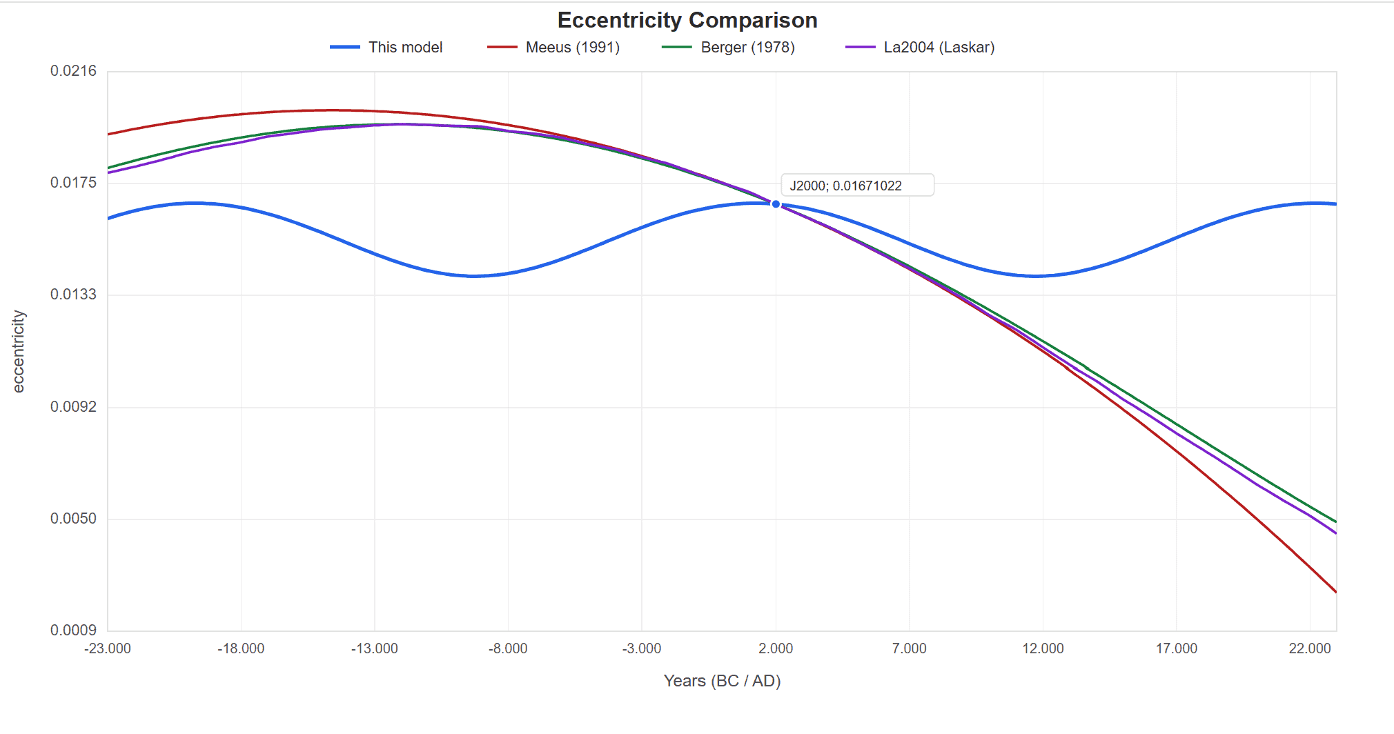
Evidence Assessment

Evidence supporting Laskar/Milankovitch:

1. Fundamental physics: Laskar’s calculations derive from Newton’s laws and observed planetary masses. The mathematics is well-established secular perturbation theory.

2. Geological proxy agreement: Ice cores, marine sediments, and speleothems all show ~100k cycles over the past million years (though with circularity concerns - see §5).

3. Spectral analysis: Climate records show power at Milankovitch frequencies (~100k, ~41k, ~23k), not at 20,868 years.

4. No 20,868-year signal in proxies: If eccentricity truly varied with 20,868-year period, this should appear in geological records. It doesn’t.

Evidence the model could invoke:

1. The 100,000-year problem is real: The dominance of ~100k over ~41k obliquity remains unexplained. Alternative explanations deserve consideration.

2. Circularity in dating: Marine sediment chronologies (LR04) and many ice core chronologies use orbital tuning, assuming Milankovitch theory. This cannot independently validate it.

3. Laskar’s predictions are unverified for deep time: Direct observations only cover ~centuries. Predictions for 10,000+ years are extrapolations.

4. The ~100k pattern may not be eccentricity: The model (and Muller & MacDonald 1997) propose the ~100k signal is inclination precession, not eccentricity.

The “Five Problems” Revisited

The eccentricity.mdx page lists “Five Problems with the Conventional Theory.” Here’s a fair assessment:

1. “No actual ~100k cycle”

• Claim: Milankovitch calculated ~95k and ~125k, not ~100k
• Assessment: Technically correct, but scientists understand this. The “~100k” refers to the combined quasi-periodic effect, not a single sine wave. This is well-documented in the literature.

2. “No ~400k pattern in data”

• Claim: Geological records don’t show ~400k periodicity
• Assessment: Partially valid. The ~400k eccentricity modulation is difficult to detect in climate records, which has led to debate about whether eccentricity directly forces climate or merely modulates precession effects. This is a genuine scientific question.

3. “Insufficient energy effect (~0.2%)”

• Claim: Eccentricity changes annual insolation too weakly to cause ice ages
• Assessment: Valid point - this is the “100,000-year problem.” However, mainstream science proposes amplification mechanisms (ice sheet dynamics, carbon feedbacks), not that eccentricity cycles don’t exist.

4. “Theoretical, not measured”

• Claim: The ~95k/~125k/~400k cycles are calculated, not observed
• Assessment: Partially valid. Direct observation of eccentricity change requires millennia. However, the physics underlying Laskar’s calculations (planetary perturbations) is well-verified by short-term planetary observations.

5. “Missing inclination precession”

• Claim: Milankovitch didn’t know about inclination precession
• Assessment: Historically interesting but not decisive. Modern orbital calculations (Laskar) do include all relevant dynamical effects. The question is whether the ~100k climate signal reflects eccentricity or inclination - a legitimate scientific debate (see Muller & MacDonald 1997).

Testable Predictions

Short-term (verifiable now): Both Laskar and the model predict decreasing eccentricity. Current measurements cannot distinguish between them.

Medium-term (~1,000 years):

• Laskar: Eccentricity continues decreasing smoothly
• Model: Eccentricity continues decreasing (both agree for this timeframe)

Long-term (~10,000+ years):

• Laskar: Minimum ~0.005 around 27,000 AD
• Model: Minimum ~0.0139 around 11,680 AD

These differences are significant but require geological timescales to verify directly.

Indirect tests (potentially shorter timeframe):

• If the model is correct, the ~100k glacial cycles should show evidence of ~111k periodicity when dated without orbital tuning
• If Laskar is correct, improved dating methods should continue to confirm ~100k timing

Honest Assessment

Strengths of the model’s approach:

1. Addresses genuine scientific problems: The 100,000-year problem is real and acknowledged by mainstream scientists. As noted by researchers: “It doesn’t make a lot of sense, because the eccentricity changes are so small, and the resulting changes in the sunlight are so small that we wouldn’t expect it to happen.” (Wikipedia: 100,000-year problem )

2. Spectral mismatch supports alternatives: Muller & MacDonald (1997)  demonstrated that the eccentricity spectrum does not match the climate spectrum:

   • Eccentricity has a split peak at ~95k and ~125k years
   • Climate records show a single narrow peak near ~100k
   • They concluded: “the shape of the peak is incompatible with both linear and nonlinear models that attribute the cycle to eccentricity”

3. The 400,000-year problem: Eccentricity’s strongest component is 400,000 years, yet this cycle is largely absent from climate records of the past 1.2 million years (Muller’s work on ice ages ). This is difficult to explain if eccentricity drives ice ages.

4. Peer-reviewed inclination support: The proposal that inclination (not eccentricity) drives the ~100k cycle was published in PNAS and matches both the spectral and bispectral fingerprints of climate data (Muller & MacDonald 1997 ).

5. Orbital tuning circularity acknowledged: Even mainstream scientists acknowledge this concern. Dr. Lisiecki of UCSB summarized: “The circular reasoning argument is the most fundamental challenge to the orbital tuning technique.” (ScienceDirect )

6. Laskar’s predictions have limitations: Due to chaotic behavior in the Solar System, Laskar’s orbital solutions are only reliable for ~50 million years (La2010 paper ). For shorter timescales, uncertainties in tidal dissipation remain “the main unknown parameter for the precession and obliquity evolution.”

7. The 21,000-year climatic precession connection: Standard astronomy recognizes that axial precession (~26k years) and apsidal precession (~112k years) combine to produce the ~21,000-year “climatic precession” cycle. The model’s 20,868-year cycle is remarkably close to this value and derives from the same principle (meeting frequency of counter-rotating motions).

Significant weaknesses (these must be acknowledged):

1. Contradicts fundamental celestial mechanics: The 20,868-year eccentricity cycle has no basis in standard orbital dynamics. Eccentricity in mainstream physics is determined by orbital energy and angular momentum, not by the meeting of precession cycles.

2. No physical derivation: The solstice-eccentricity correlation lacks physical explanation. Why would Earth’s axial orientation affect its orbital shape?

3. Missing signal in proxies: No clear 20,868-year periodicity appears in geological records. If eccentricity truly varied with this period, it should be detectable.

4. Much narrower range: The model’s 0.003 range (0.0139-0.0167) contradicts geological evidence suggesting much larger past variations (0.0005-0.058). However, this evidence comes from orbitally-tuned records (see circularity concern).

5. Geological proxies: While the ~100k signal might be inclination rather than eccentricity (supporting the model’s climate argument), this doesn’t explain why the measured astronomical eccentricity follows Laskar’s predictions in recent centuries.

Counter-arguments the model must address:

1. Why does Muller & MacDonald’s ~100k inclination match climate data, while the model claims ~111k? The model needs to explain this 10% discrepancy, either through dating errors or by distinguishing its claim from Muller’s.

2. Telescopic observations: Modern precise measurements of Earth’s orbital elements match Laskar’s calculations. How does the model reconcile its 20,868-year cycle with these observations?

3. The mechanism question: Even if eccentricity doesn’t drive ice ages (supporting inclination), this doesn’t prove the model’s 20,868-year eccentricity cycle exists. These are separate claims.

The key challenge: The model’s eccentricity claim requires either:

• Demonstrating that Laskar’s fundamental physics is wrong (extraordinary claim requiring extraordinary evidence)
• Or showing that the model’s “eccentricity” refers to an apparent or observational effect rather than true orbital eccentricity (in which case terminology should be clarified)
• Or providing a physical mechanism connecting precession alignment to orbital shape changes

Connection to Ice Core Chronology (§5)

The model’s eccentricity claim is linked to its ice core argument:

The model proposes:

1. The ~100k glacial signal is actually ~111k (inclination precession)
2. Ice core dating has ~10% systematic error from orbital tuning
3. The model’s 20,868-year eccentricity cycle is separate from the glacial ~100k pattern

Implication: If the model is correct about ice core chronology, it would support reinterpreting the ~100k climate signal as inclination rather than eccentricity. This doesn’t directly validate the 20,868-year eccentricity cycle, but it removes one objection (that ~100k proxies contradict it).

See §5 (Ice Core Chronology) for detailed analysis of dating methods and the circularity problem.

Summary

The model’s eccentricity claim is its most challenging assertion because it contradicts well-established celestial mechanics. The current scientific evidence strongly favors Laskar’s predictions, though the “100,000-year problem” shows that the climate implications of orbital variations remain debated

5. Ice Core Chronology

This section examines ice core dating methods and their relevance to the model’s claim that the ~100,000-year glacial cycle is actually ~111,296 years (the inclination precession period).

The Model’s Claim

The Holistic Universe Model proposes that the dominant ~100,000-year pattern in glacial-interglacial cycles reflects the inclination precession period (~111,296 years), not Milankovitch’s eccentricity cycles (~95k/~125k). This would require that ice core chronologies have a systematic error of ~10% for older ice.

This is a significant claim that deserves careful examination.

How Ice Cores Are Dated

Modern ice core chronology uses multiple independent methods:

1. Annual layer counting (most precise for recent ice):

• Visual stratigraphy (summer/winter layers)
• Chemical signatures (seasonal dust, sea salt, isotopes)
• Electrical conductivity measurements (ECM)
• Precision: ±1% for Holocene (~11,700 years), ±2-3% for glacial periods
• Limitation: Layers become too thin to resolve beyond ~60,000-100,000 years

2. Volcanic markers (absolute tie points):

• Sulfate spikes from known eruptions
• Tephra (volcanic ash) layers with unique chemical signatures
• Examples: Toba (74 ka), Laacher See (12.9 ka), Campanian Ignimbrite (39 ka)
• Strength: Provides independent absolute dates where identified

3. Gas synchronization (global correlation):

• Methane (CH₄) variations are globally synchronous (within ~50 years)
• Links Greenland and Antarctic records precisely
• Allows transfer of well-dated Greenland chronology to Antarctic cores
• Precision: ±50-200 years for the synchronization itself
• Limitation: Still requires one record to have an independent chronology

4. O₂/N₂ ratio dating (Kawamura et al. 2007 ):

• Trapped air’s O₂/N₂ ratio correlates with local summer insolation
• Provides an independent orbital constraint without assuming eccentricity cycles
• Used to validate AICC2012 chronology for Dome Fuji core
• Key feature: This method constrains timing to precession cycles (~23 ka), not ~100 ka cycles

5. Radiometric dating (uranium-series, ¹⁴C):

• Radiocarbon (¹⁴C) useful to ~50 ka
• U-series dating of speleothems synchronized to ice cores
• Strength: Completely independent of orbital assumptions

6. Orbital tuning (matches isotopes to insolation):

• Adjusts chronology so δ¹⁸O variations match calculated insolation changes
• Assumes Milankovitch theory is correct
• Critical issue: This method is circular if used to test Milankovitch theory!

Major Ice Core Chronologies

AICC2012 (Antarctic Ice Core Chronology 2012) is the current community standard for long Antarctic records. It uses:

• Layer counting where possible
• Gas synchronization between cores
• Glaciological ice flow modeling
• Minimal orbital tuning (only for transitions where other constraints are weak)

Chronology Uncertainties

The Circularity Problem

Standard orbital tuning works by adjusting the ice core timescale so that δ¹⁸O (ice isotope) variations match calculated summer insolation at high latitudes. This assumes:

1. Climate responds predictably to insolation
2. Milankovitch’s insolation calculations are correct
3. The response time (phase lag) is known

This is circular when testing Milankovitch theory. If you tune your chronology to match Milankovitch predictions, you cannot then use that chronology to validate Milankovitch theory.

The model’s argument: If chronologies are orbitally tuned assuming ~100k eccentricity cycles, they would artificially compress a true ~111k signal to appear as ~100k.

Counter-argument: Modern chronologies (especially AICC2012) minimize orbital tuning:

• Use multiple independent constraints
• Only apply tuning where other methods fail
• The O₂/N₂ method constrains precession timing independently
• Volcanic markers provide absolute tie points unaffected by tuning

The Key Question: How Much Does Tuning Affect the ~100k Pattern?

For the model’s claim to hold (that ~100k is actually ~111k), the following would need to be true:

1. Systematic error of ~10%:

• 111,296 / 100,000 = 1.11 (11% difference)
• All major ice core chronologies would need this same systematic bias

2. Affects multiple independent records:

• Antarctic (EPICA, Vostok, Dome Fuji)
• Greenland (NGRIP, GRIP, GISP2)
• Marine sediment cores (which have their own dating methods)

3. Not detected by non-orbital methods:

• Volcanic markers
• Radiometric dating
• U-series speleothem correlations

Evidence Assessment

Evidence supporting conventional ~100k chronology:

1. Multiple independent methods converge: Layer counting, volcanic markers, gas synchronization, and U-series correlations all support the established chronology within their uncertainty bounds.

2. O₂/N₂ dating (Kawamura et al. 2007 ): This method uses precession cycles (~23 ka), not ~100k cycles, to constrain timing. It validates the AICC2012 chronology independently.

3. Speleothem correlations (Cheng et al. 2016 ): Cave deposits dated by U-Th (completely independent of ice) show the same ~100k pattern with consistent timing.

4. Marine sediment records (Lisiecki & Raymo 2005 ): The LR04 stack of 57 benthic δ¹⁸O records shows ~100k cycles, using multiple dating methods including biostratigraphy and magnetostratigraphy.

Evidence the model could invoke:

1. Orbital tuning is still used: Even AICC2012 applies some orbital tuning for ice older than ~400 ka, where other methods are limited.

2. The “100,000-year problem” is real: The dominance of ~100k cycles over the expected ~41k obliquity signal has puzzled scientists since the 1970s. The mechanism is still debated.

3. Marine δ¹⁸O also uses orbital tuning: The LR04 stack (Lisiecki & Raymo 2005 ) explicitly uses orbital tuning, so it cannot independently confirm ice core chronology.

4. Spectral analysis shows spread: The “~100k” peak in spectral analyses typically spans 80-120 ka, which could accommodate either ~100k or ~111k.

5. Peer-reviewed support for inclination hypothesis: Muller & MacDonald (1997) argued in PNAS that orbital inclination, not eccentricity, drives the ~100k glacial cycle (see below).

The Inclination Hypothesis (Muller & MacDonald 1997)

The model’s claim that the ~100k glacial signal reflects inclination precession is not unique. A peer-reviewed hypothesis in the Proceedings of the National Academy of Sciences made a similar argument:

Muller & MacDonald (1997) : “Spectrum of 100-kyr glacial cycle: Orbital inclination, not eccentricity”

Key findings:

1. Spectral mismatch with eccentricity: The observed ~100k peak in climate data is narrow and well-defined. However, the eccentricity spectrum shows peaks at ~95k and ~125k years - not a single ~100k peak. The climate data doesn’t match eccentricity’s spectral shape.

2. Inclination provides better match: Earth’s orbital inclination relative to the invariable plane (perpendicular to the solar system’s angular momentum vector) has a dominant ~100k period that closely matches the climate spectrum.

3. Bispectral analysis: The authors found that the bispectrum (which reveals phase relationships between frequency components) of the climate data matches the inclination signal, but not eccentricity.

4. Proposed mechanism: The authors suggested extraterrestrial accretion (meteoroids or interplanetary dust) as the link between inclination and climate - though this mechanism remains speculative.

Relevance to the model:

Important distinction: Muller & MacDonald found that inclination changes match the ~100k climate signal as currently dated. The Holistic Universe Model goes further, proposing that the true period is ~111k and the ~100k appearance is a dating artifact. These are related but distinct claims.

Status of the Muller-MacDonald hypothesis: This hypothesis remains controversial. While the spectral analysis is sound, the proposed mechanism (extraterrestrial accretion) has not been confirmed, and most paleoclimatologists still favor explanations involving eccentricity modulation of precession. However, the “100,000-year problem” remains unresolved, and the Muller-MacDonald work demonstrates that serious scientists have questioned the eccentricity explanation.

Honest Assessment

For the model’s claim (that ~100k is actually ~111k):

The model would need to explain why:

• Multiple independent dating methods all have the same ~10% systematic bias
• O₂/N₂ dating (which doesn’t use ~100k cycles) still supports the established chronology
• Volcanic markers (absolute dates) don’t reveal the discrepancy
• The error is consistent across Antarctic, Greenland, and marine records

Strengths of the claim:

• The “100,000-year problem” shows that the ~100k pattern isn’t well explained by eccentricity
• Orbital tuning creates real circularity concerns
• The spectral peak is broad enough that ~111k isn’t strictly excluded

Weaknesses of the claim:

• No proposed mechanism for systematic bias across all dating methods
• Independent methods (U-series, ¹⁴C, volcanic markers) support conventional chronology
• The ~10% error is at the very upper limit of uncertainty estimates
• Recent cycles (<400 ka) have better constraints and still show ~100k pattern

What Would Test This?

If the model is correct:

1. Future improvements in ice core dating (better volcanic correlations, new radiometric methods) should reveal systematic offsets
2. The ~100k pattern should show slight stretching when dated without orbital tuning
3. Marine sediment records dated without tuning should show ~111k rather than ~100k

If the conventional chronology is correct:

1. New dating methods should continue to validate existing chronologies
2. The ~100k spectral peak should tighten with better data, not shift toward ~111k
3. Independent speleothem and marine records should maintain ~100k timing

Connection to the Model

The Holistic Universe Model proposes:

• The ~100k glacial pattern reflects inclination precession (~111,296 years)
• This is the period of Earth’s orbital plane tilting relative to the invariable plane
• The ~10% discrepancy is within (upper) dating uncertainties

See Eccentricity for the model’s full explanation of why the ~100k signal may reflect inclination precession rather than eccentricity cycles.

Summary

The model’s claim is scientifically testable but faces significant challenges. The current evidence favors conventional chronology, though the “100,000-year problem” shows that the underlying climate mechanism remains debated.

6. Mathematical Framework

Coordinate System Definitions

ICRS (International Celestial Reference System):

• Origin: Solar system barycenter
• X-axis: Toward vernal equinox (J2000)
• Z-axis: Toward celestial north pole (J2000)
• Fixed relative to distant quasars

Model Reference Points:

EARTH-WOBBLE-CENTER:

• Definition: A reference point that Earth orbits around, used to simulate the axial precession “wobble”

• Location: At the center of Earth’s Axial Precession Orbit (APO), approximately 213,000 km from Earth’s center (0.001431 AU)

• Motion: Earth orbits this point clockwise (as viewed from above the North Pole) in ~25,684 years

• Physical interpretation: Represents the combined gravitational torque from Moon and Sun that causes Earth’s axis to precess

• Mathematical representation: In the 3D simulation, Earth is placed at orbital radius 0.001431 AU from this center point

• Derivation of the 0.001431 AU value: This is a calibrated model parameter, not a directly measured distance. It was determined by:

  1. Setting the orbital period to ~25,684 years (mean axial precession)
  2. Requiring the simulation to produce correct precession rate (~50.29″/year)
  3. Iterating the radius until the obliquity variation amplitude matches observations (~0.634°)

  The value has no independent physical meaning - it’s the radius that makes the mathematical model reproduce observed precession behavior. Think of it as similar to how Ptolemy’s epicycle radii were calibrated to match planetary positions without corresponding to physical objects.

PERIHELION-OF-EARTH:

• Definition: A reference point near the Sun that represents the center of Earth’s elliptical orbit and the direction of Earth’s perihelion
• Location: Orbits the Sun at radius ~2,292,000 km (0.015321 AU) - this is the base eccentricity (arithmetic midpoint of the eccentricity cycle; the time-averaged mean is 0.015387)
• Motion: Orbits the Sun counter-clockwise (prograde) in ~111,296 years
• Physical interpretation: Represents Earth’s apsidal precession - the slow rotation of Earth’s orbital ellipse due to planetary perturbations (mainly Jupiter)
• Mathematical representation: In the 3D simulation, this point’s angular position determines Earth’s longitude of perihelion

Derivation of Key Periods

The Holistic Universe Model derives all precession cycles from a single master period: 333,888 years (the “Holistic-Year”). This value is determined empirically by fitting to the observed axial precession period.

Step 1: Starting from observed axial precession

The IAU 2006 precession constant gives:

Observed precession rate = 50.2879"/year (with small corrections)

This yields an instantaneous axial precession period of approximately 25,772 years. However, this rate varies over time due to changing obliquity. The model derives its base value from the mean rate:

Axial precession (mean) ≈ 25,683.69 years

Step 2: Deriving the Holistic-Year

The model proposes that precession cycles follow Fibonacci ratios. Given axial precession corresponds to the Fibonacci number 13:

Holistic-Year = 25,683.69 × 13 = 333,888 years

Step 3: Deriving other periods

All other cycles follow from dividing by Fibonacci numbers:

Note on Fibonacci sequence: 1, 1, 2, 3, 5, 8, 13, 21, 34… The divisors 3, 8, 13, 16 are from this sequence (16 = 13 + 3, a Fibonacci-like combination). See Formula Derivation: Fibonacci Hierarchy for how this pattern extends to planetary cycles.

Core Simulation Equations

The 3D simulation calculates orbital parameters using these relationships:

1. Obliquity (axial tilt)

ε(t) = ε₀ + A × [-cos(2π(t-t₀)/P₃) + cos(2π(t-t₀)/P₈)]

Where:
  ε₀ = 23.41398° (mean obliquity)
  A  = 0.633849° (amplitude)
  P₃ = 333,888/3 = 111,296 years (inclination precession)
  P₈ = 333,888/8 = 41,736 years (obliquity cycle)
  t₀ = -301,340 (anchor year)

2. Orbital inclination (to invariable plane)

i(t) = i₀ - A × cos(2π(t-t₀)/P₃)

Where:
  i₀ = 1.481592° (mean inclination)
  A  = 0.633849° (same amplitude as obliquity)
  P₃ = 111,296 years

3. Eccentricity

The eccentricity formula is more complex, involving the meeting frequency of two counter-rotating motions:

Meeting period = 1 / (1/P₁₃ + 1/P₃) = P₁₆

Where:
  P₁₃ = 25,683.69 years (axial precession, clockwise)
  P₃  = 111,296 years (inclination precession, counter-clockwise)
  P₁₆ = 20,868 years (resulting eccentricity cycle)

The full eccentricity equation (see Formulas) produces values oscillating between ~0.0139 and ~0.0167.

4. Longitude of perihelion

λ(t) = 270° + 360°(t-t₀)/P₁₆ + corrections

With sinusoidal corrections for the apsidal motion.

Comparison with Standard Formulas

Key observation: The model matches current observed values well, but diverges significantly from Laskar/Berger predictions for deep time. Both approaches are theoretical extrapolations that cannot be directly verified for ancient/future periods.

Error Analysis

Sources of uncertainty in model calculations:

1. Anchor year (t₀ = -301,340)

• Derived by fitting to J2000 observed values
• Uncertainty: The anchor year is not independently constrained
• Effect: Shifts phase of all cycles but not periods

2. Amplitude (A = 0.633849°)

• Derived from observed obliquity range
• Current observed range: 22.1° to 24.5° over ~41,000 years
• Model predicts: 22.21° to 24.71° (combined range from two ±0.634° components)
• Uncertainty: ±0.01° based on current measurements

3. Mean values

• Mean obliquity (23.41398°): Based on IAU J2000 value, uncertainty <0.001°
• Base eccentricity (0.015321): Model-derived arithmetic midpoint of eccentricity cycle (time-averaged mean = 0.015387)

4. Period uncertainties

*Note: Standard theory doesn’t define “inclination precession” in the same way. The closest comparison is Earth’s nodal precession relative to the invariable plane, which differs significantly.

Propagated uncertainty in predictions:

For J2000 + 1000 years (year 3000):

• Obliquity: Model predicts 23.53° ± 0.02°
• Eccentricity: Model predicts 0.0166 ± 0.0001

For J2000 + 10,000 years (year 12000):

• Obliquity: Model predicts 22.41° ± 0.2°
• Eccentricity: Model predicts 0.0142 ± 0.001

Comparison with Laskar predictions:

Important caveat: Agreement with Laskar over the next ~10,000 years doesn’t validate the model, as both are extrapolations from similar J2000 starting conditions. Significant divergence only appears beyond ~50,000 years.

Short-Term Perturbations

The model describes long-term cycles (thousands to hundreds of thousands of years). A valid question is: how does it handle short-term variations (years to decades)?

What the Model Includes

The model explicitly includes:

What the Model Does NOT Include

Why These Are Omitted

1. The model describes secular (long-term) trends only

The model’s equations produce smooth curves representing mean values over the precession cycles. Short-term oscillations are considered “noise” around these secular trends.

Analogy: Climate models distinguish between:

• Weather (short-term variations, days to weeks)
• Climate (long-term averages, decades to millennia)

Similarly, the Holistic Universe Model describes “orbital climate” (secular trends) not “orbital weather” (short-term perturbations).

2. Short-term effects average to zero

Over timescales longer than the perturbation period, these effects average out:

• The 18.6-year nutation averages to zero over ~40 years
• Jupiter’s ~12-year perturbations average out over ~100 years
• The Chandler wobble averages to zero over ~10 years

3. Practical impact is small

For the model’s primary predictions (obliquity, eccentricity, longitude of perihelion over millennia), short-term perturbations contribute:

• < 0.01° to obliquity predictions
• < 0.0001 to eccentricity predictions
• < 0.1° to longitude predictions

These are within the model’s stated uncertainties.

Comparison with Standard Astronomy

Standard astronomical ephemerides (JPL DE440/441) include all these perturbations through numerical integration. This is why DE440/441 achieves sub-arcsecond precision for short timescales.

The Holistic Universe Model is not designed to compete with ephemerides for short-term predictions. Its purpose is to:

1. Provide a unified framework for understanding long-term precession cycles
2. Make predictions about millennial-scale trends
3. Offer an alternative interpretation of the Fibonacci ratios in these cycles

For precise positions on any given day, use JPL Horizons. For understanding the ~26,000-year and ~111,000-year cycles, the model provides a conceptual framework.

What This Means for Testability

Short-term tests are difficult because short-term perturbations mask the secular trends. The model’s predictions become testable when:

1. Averaging over sufficient time to remove short-term noise (decades to centuries)
2. Comparing with other long-term models (Laskar, Berger) rather than daily ephemerides
3. Focusing on phenomena where short-term perturbations don’t dominate (e.g., eccentricity minimum timing)

Calibration Transparency

A common criticism of phenomenological models is circular reasoning: if you tune parameters to match data, then cite that match as evidence, you’ve proven nothing. This section explicitly addresses this concern.

The Circularity Problem

The concern (valid):

“If 333,888 was found by fitting to observations, then claiming the model ‘matches observations’ is meaningless. You’ve just done curve-fitting.”

This is a legitimate scientific concern. Any model with adjustable parameters can be made to fit data. The question is: what can the model predict that it wasn’t trained on?

Degrees of Freedom Analysis

The model has 5 adjustable parameters:

For comparison:

• Laskar’s (1993) obliquity formula has ~6 free parameters
• Standard precession theory uses multiple fitted constants

The model has a similar number of free parameters to standard approaches.

What Was Used to Find 333,888?

Direct inputs (the model was explicitly fitted to these):

1. J2000 year lengths - Only H ≈ 333,888 produces solar year (365.242190 days) and sidereal year (365.256363 days) matching observations. See Days & Years for how these derive from obliquity and eccentricity.
2. 1246 AD perihelion-solstice alignment - From Meeus’s formula
3. J2000 longitude of perihelion (102.95°) - The progression from 90° to 102.95° over 754 years
4. J2000 obliquity (23.439°) - For setting mean value
5. Observed obliquity range (~22.1° to ~24.5°) - For setting amplitude

What Was NOT Used?

Genuine predictions (these values were NOT used in calibration):

Important: The eccentricity and inclination values were checked AFTER 333,888 was determined. They were not used in the fitting process.

The Climate Cycle Question

Problematic: The “eight constraints” in Mathematical Foundations include “Climate Cycles (3 × ~100k pattern)”. This is potentially circular:

1. If ~100k climate cycles were used to find 333,888 → Cannot use them as validation
2. If they were checked afterward → Valid validation

Honest answer: The climate cycle pattern was known to the author when searching for 333,888. It was part of the motivation for the search. However, the model doesn’t match the conventional ~100k; it proposes ~111k. The model’s claim is that conventional chronology has a ~10% systematic error.

This is neither purely input nor purely prediction - it’s a reinterpretation of existing data.

What Would Constitute Independent Validation?

The model can be tested by observations that:

1. Were not used in calibration
2. Cannot be adjusted after the fact
3. Differ meaningfully from standard theory

Strong tests:

Weak tests (similar predictions):

Honest Assessment

What the model CANNOT claim:

• That matching J2000 values validates the model (they were inputs)
• That matching the ~100k climate cycle validates the model (it was known during construction)
• That any parameter fitted to data constitutes evidence

What the model CAN claim:

• Obliquity predictions at dates other than J2000 agree with Laskar
• Perihelion longitude predictions at dates other than 1246 AD/J2000 agree with Meeus
• Eccentricity and inclination emerge from the structure without being used as inputs

Scientific standard: The model should be judged by its testable predictions that differ from standard theory, not by how well it reproduces data used in its construction.

7. Open Questions

The model acknowledges several unresolved questions:

Fundamental Questions

1. Why Do Fibonacci Ratios Appear in Precession Cycles?

The model proposes that Earth’s precession cycles follow Fibonacci ratios (3, 8, 13, 16). While the model fits observed data well, why these ratios appear is not explained by known physics.

The observation:

Inclination precession : Axial precession = 111,296 : 25,684 ≈ 4.33 : 1 = 13 : 3
Obliquity cycle : Perihelion precession = 41,736 : 20,868 = 2 : 1 = 8 : 4 (Fibonacci-related)

Fibonacci patterns in nature - supporting context:

The model’s author notes that Fibonacci ratios appear throughout nature and the solar system. This is not unique to the Holistic Universe Model:

Fibonacci in the solar system:

A 1968 study by A.M. Molchanov in Icarus analyzed orbital period ratios across the solar system and found that many planetary orbital resonances approximate Fibonacci fractions. More recent work has confirmed this pattern:

Aschwanden (2018)  analyzed 75 orbital period ratios in the solar system (planets and moons) and found that approximately 60% match Fibonacci fractions within measurement uncertainty.

Possible explanations:

1. Orbital resonance and stability: Fibonacci ratios may emerge naturally from gravitational resonance. Systems that settle into Fibonacci-like ratios may be more stable over billions of years. This is related to the KAM theorem (Kolmogorov-Arnold-Moser) in dynamical systems theory.

2. Golden ratio in stable systems: The golden ratio (φ ≈ 1.618, limit of Fibonacci ratios) is the “most irrational” number - hardest to approximate by simple fractions. Orbits with golden-ratio-related periods avoid destabilizing resonances.

3. Coincidence: The ratios might be approximate coincidences. The human tendency to find patterns (apophenia) may overstate the significance.

4. Selection effect: We observe the current solar system because it’s stable. Unstable configurations would have been disrupted long ago. This doesn’t explain why Fibonacci specifically, but explains why we see stable ratios.

The model’s position: The model notes that if the solar system is a “balanced system” - gravitationally relaxed over 4.5 billion years - Fibonacci ratios may emerge naturally. However, the model does not derive these ratios from first principles; they are empirically fitted.

Scientific status: Fibonacci patterns in orbital mechanics are documented in peer-reviewed literature. The specific claim that Earth’s precession cycles follow exact Fibonacci divisors of 333,888 years is not supported by mainstream astronomy. This remains an open question requiring either:

• A physical derivation from gravitational dynamics
• High-precision measurements confirming the exact periods
• Or demonstration that the apparent pattern is coincidental

2. Why Are the Amplitudes Equal (~0.634°)?

The model uses the same amplitude (0.633849°) for both:

• Axial tilt variation (obliquity oscillation)
• Orbital inclination variation (relative to the invariable plane)

The observation:

Obliquity range: 22.78° to 24.05° (amplitude 0.634°)
Inclination range: 0.848° to 2.115° (amplitude 0.634°)

This equality produces the observed obliquity behavior when both components combine in the model’s formula:

ε(t) = 23.41398° + 0.634° × [-cos(inclination phase) + cos(obliquity phase)]

Why might this be significant?

1. Conservation principle: Equal amplitudes could indicate energy or angular momentum being exchanged between the two oscillation modes. In coupled oscillator systems, equal amplitudes sometimes emerge from conservation laws.

2. Coincidence: The equality might be approximate and not exact. Current measurements may not be precise enough to detect small differences.

3. Calibration artifact: The model derives both amplitudes by fitting to the same observed obliquity range (~22.1° to ~24.5°). The equality might be an artifact of this fitting procedure rather than a physical constraint.

Comparison with standard theory:

Standard orbital mechanics calculates obliquity and inclination variations independently:

• Obliquity: ~22.1° to ~24.5° over ~41,000 years (Laskar)
• Inclination (to ecliptic): ~0° to ~3° over ~100,000 years

Standard theory does not predict equal amplitudes; the similarity in the model is a feature of its mathematical construction.

Scientific status: The equal amplitude assumption is not derived from physical principles. It is a simplifying assumption that fits current data well but may not hold over longer timescales.

3. Why 333,888 Years Specifically?

The Holistic-Year (333,888 years) is an empirically fitted value, not a derived constant.

The fitting process:

The model establishes that year lengths depend on orbital parameters (see Days & Years for details):

• The sidereal year in seconds is fixed (Earth’s orbital period relative to fixed stars)
• Obliquity drives the solar year length
• Eccentricity drives the sidereal year in days
• Day length = sidereal year (seconds) / sidereal year (days)

The 3D simulation calculates year lengths for any Holistic-Year value. When testing different values, only H ≈ 333,888 produces year lengths matching J2000 observations:

• Solar year: 365.242190 days
• Sidereal year: 365.256363 days

The Fibonacci connection:

The value 333,888 ≈ 25,684 × 13, where 25,684 is the mean axial precession period and 13 is a Fibonacci number. This relationship fits the model’s Fibonacci-fraction pattern for orbital periods, but remains unexplained — it is an observation, not a derivation.

Testable Questions

4. Will Mercury’s “Anomaly” Change?

• Model predicts decrease from ~40 to ~34″/century over ~5,000 years
• Current measurements show no drift (uncertainty ~0.003″/century/decade)
• Requires continued precision observation
• See Mercury Precession for full analysis

5. Will Eccentricity Follow the 20,868-Year Cycle?

• Model predicts minimum eccentricity (~0.0139) around 11,680 AD
• Laskar predicts continued slow decrease toward ~0.005 over millions of years
• Testable over geological timescales through proxy records
• Near-term (next few millennia): both predictions similar; divergence grows with time

6. Will Axial Precession Rate Reverse Its Trend?

• Model predicts precession rate maximum soon, then decrease
• Standard theory (Capitaine et al.) predicts continued decrease
• Current rate: ~50.29″/year (decreasing at ~0.0002″/year²)
• Model predicts reversal within ~2,000 years
• Testable with VLBI precision within decades

8. References

Primary Sources Used in the Model

1. Precession theory:

   • Capitaine, N., Wallace, P.T., & Chapront, J. (2003). “Expressions for IAU 2000 precession quantities.” Astronomy & Astrophysics, 412, 567-586.

2. Obliquity calculations:

   • Laskar, J., Robutel, P., Joutel, F., et al. (2004). “A long-term numerical solution for the insolation quantities of the Earth.” Astronomy & Astrophysics, 428, 261-285.
   • Laskar, J. (1993). “Orbital, precessional and insolation quantities for the Earth from -20 Myr to +10 Myr.” Astronomy & Astrophysics, 270, 522-533.
   • Vondrák, J., Capitaine, N., & Wallace, P. (2011). “New precession expressions, valid for long time intervals.” Astronomy & Astrophysics, 534, A22. Link 

3. Perihelion calculations:

   • Meeus, J. (1998). Astronomical Algorithms (2nd ed.). Willmann-Bell.

4. Invariable plane:

   • Souami, D., & Souchay, J. (2012). “The solar system’s invariable plane.” Astronomy & Astrophysics, 543, A133.

5. Planetary ephemerides:

   • Park, R.S., et al. (2021). “The JPL Planetary and Lunar Ephemerides DE440 and DE441.” The Astronomical Journal, 161, 105.

Climate and Ice Core References

6. Milankovitch theory:

   • Hays, J.D., Imbrie, J., & Shackleton, N.J. (1976). “Variations in the Earth’s orbit: Pacemaker of the ice ages.” Science, 194, 1121-1132.

7. 100,000-year problem:

   • Imbrie, J., et al. (1993). “On the structure and origin of major glaciation cycles.” Paleoceanography, 8(6), 699-735.

8. Ice core chronology:

   • Veres, D., et al. (2013). “The Antarctic ice core chronology (AICC2012): an optimized multi-parameter and multi-site dating approach for the last 120 thousand years.” Climate of the Past, 9, 1733-1748. Link 
   • Parrenin, F., et al. (2007). “The EDC3 chronology for the EPICA Dome C ice core.” Climate of the Past, 3, 485-497. Link 
   • Rasmussen, S.O., et al. (2014). “A stratigraphic framework for abrupt climatic changes during the Last Glacial period based on three synchronized Greenland ice-core records.” Quaternary Science Reviews, 106, 14-28.
   • Kawamura, K., et al. (2007). “Northern Hemisphere forcing of climatic cycles in Antarctica over the past 360,000 years.” Nature, 448, 912-916. Link 

9. Marine sediment chronology:

   • Lisiecki, L.E., & Raymo, M.E. (2005). “A Pliocene-Pleistocene stack of 57 globally distributed benthic δ¹⁸O records.” Paleoceanography, 20, PA1003. Link 

10. Speleothem chronology:

    • Cheng, H., et al. (2016). “The Asian monsoon over the past 640,000 years and ice age terminations.” Science, 352, 343-347.

11. Inclination hypothesis:

    • Muller, R.A., & MacDonald, G.J. (1997). “Spectrum of 100-kyr glacial cycle: Orbital inclination, not eccentricity.” Proc. Natl. Acad. Sci. U.S.A., 94(16), 8329-8334. Link 

12. Milankovitch original work:

    • Milankovitch, M. (1941). Canon of Insolation and the Ice-Age Problem. Royal Serbian Academy Special Publication 132. (English translation: Israel Program for Scientific Translations, 1969)

13. Modern orbital solutions:

    • Laskar, J., Fienga, A., Gastineau, M., & Manche, H. (2011). “La2010: A new orbital solution for the long-term motion of the Earth.” Astronomy & Astrophysics, 532, A89. Link 

14. 100,000-year problem mechanisms:

    • Raymo, M.E. (1997). “The timing of major climate terminations.” Paleoceanography, 12(4), 577-585.
    • Paillard, D. (1998). “The timing of Pleistocene glaciations from a simple multiple-state climate model.” Nature, 391, 378-381. Link 
    • Raymo, M.E., Lisiecki, L.E., & Nisancioglu, K.H. (2006). “Plio-Pleistocene Ice Volume, Antarctic Climate, and the Global δ¹⁸O Record.” Science, 313, 492-495.

Mercury Perihelion References

15. Historical:

    • Le Verrier, U.J. (1859). “Lettre de M. Le Verrier à M. Faye sur la théorie de Mercure.” Comptes Rendus, 49, 379-383.
    • Newcomb, S. (1882). Astronomical Papers of the American Ephemeris, Vol. 1.
    • Clemence, G.M. (1947). “The Relativity Effect in Planetary Motions.” Reviews of Modern Physics, 19, 361.

16. Modern measurements:

    • Park, R.S., et al. (2017). “Precession of Mercury’s Perihelion from Ranging to the MESSENGER Spacecraft.” The Astronomical Journal, 153, 121. Link 

17. Academic critiques:

    • Křížek, M., & Somer, L. (2023). Mathematical Aspects of Paradoxes in Cosmology. Springer. Link 
    • Křížek, M. (2015). “On the Perihelion Precession.” PDF 

Fibonacci and Orbital Resonance References

18. DNA and Golden Ratio:

    • Yamagishi, M.E.B., & Shimabukuro, A.I. (2008). “Nucleotide frequencies in human genome and Fibonacci numbers.” Bull. Math. Biol., 70(3), 643-653. PubMed 

19. Phyllotaxis (plant Fibonacci patterns):

    • Prusinkiewicz, P., & Lindenmayer, A. (1990). The Algorithmic Beauty of Plants. Springer. Link 

20. Planetary orbital resonances:

    • Molchanov, A.M. (1968). “The resonant structure of the Solar System.” Icarus, 8(1-3), 203-215. ScienceDirect 

21. Solar system Fibonacci analysis:

    • Aschwanden, M.J. (2018). “Self-organizing systems in planetary physics: Harmonic resonances of planet and moon orbits.” New Astronomy, 58, 107-123. arXiv 

Last updated: January 2026

Return to Mathematical Foundations | Predictions | Formulas